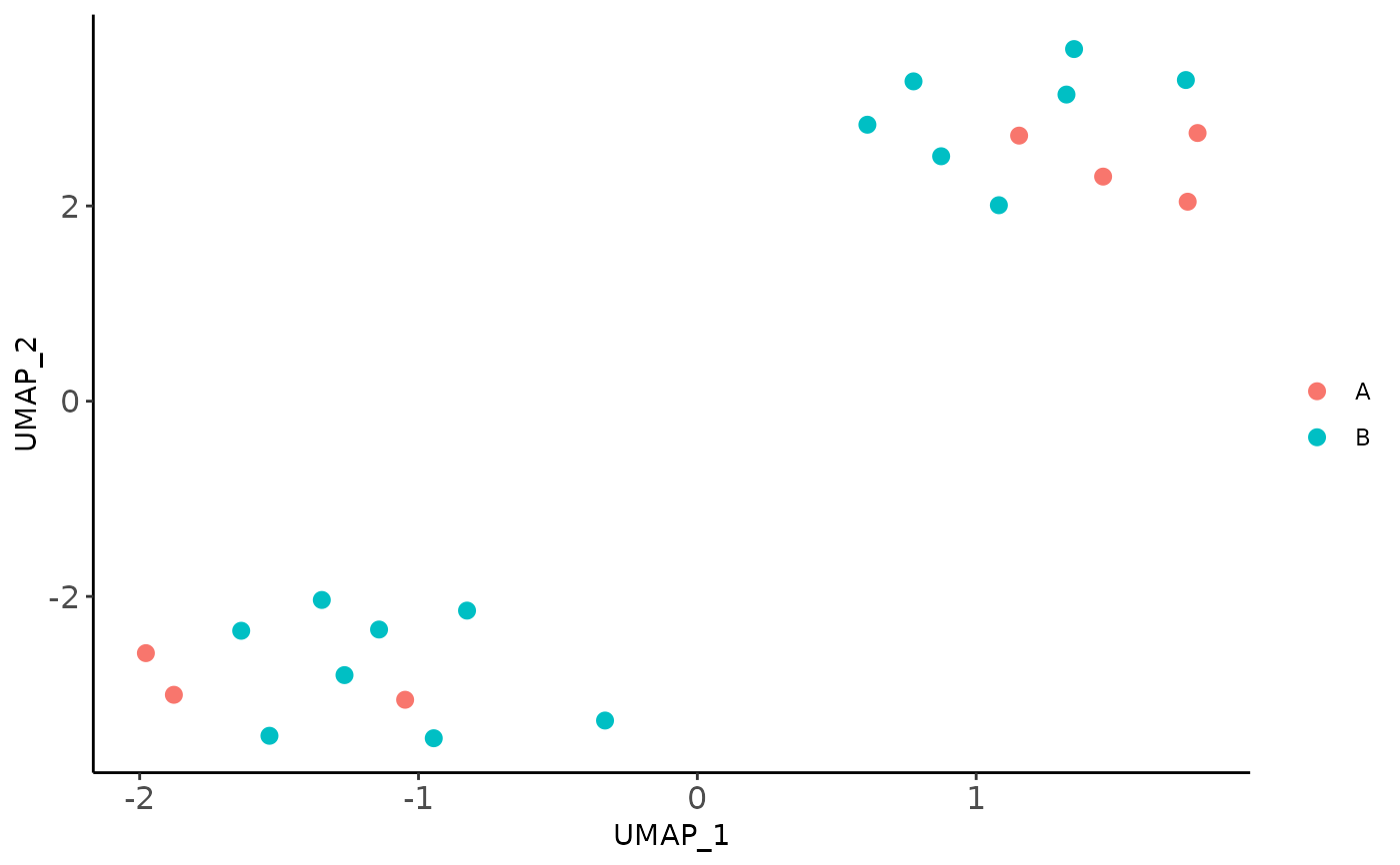
Visualize sample variability in a 2D space — plot_sample

Performs dimensionality reduction of factor scores for the visualization of sample-level variability

Usage

plot_sample_2D(
  model,
  group = FALSE,
  method = "UMAP",
  metadata,
  sample_id_column = "sample",
  color_by,
  ...
)

Arguments

model: A MOFA2 model.
group: Boolean flag TRUE/FALSE, to specify if a grouped MOFA model is provided.
method: A string specifying if "UMAP" or "MDS" should be performed
metadata: A data frame containing the annotations of the samples included in the MOFA model.
sample_id_column: A string character that refers to the column in metadata where the sample identifier is located.
color_by: A string character that refers to the column in metadata where the covariate to be tested is located.
...: inherited parameters of uwot::umap()

Value

A dataframe in a tidy format containing the manifold and the scatter plot

Details

For a MOFA2 model it performs a multidimensional scaling (MDS) or uniform manifold approximation and projection (UMAP) of the factor scores. It allows you to color samples based on a covariate available in your meta-data.

Examples

inputs_dir <- base::system.file("extdata", package = "MOFAcellulaR")
model <- MOFA2::load_model(file.path(inputs_dir, "testmodel.hdf5"))
#> Warning: Factor(s) 1 are strongly correlated with the total number of expressed features for at least one of your omics. Such factors appear when there are differences in the total 'levels' between your samples, *sometimes* because of poor normalisation in the preprocessing steps.
metadata <- readRDS(file.path(inputs_dir, "testmetadata.rds"))
UMAP_embedding <- plot_sample_2D(model = model,
                                 group = FALSE,
                                 method = "UMAP",
                                 metadata = metadata,
                                 sample_id_column = "sample",
                                 color_by = "batch")