PHONEMeS follows the pipeline that is depicted in the following figure:
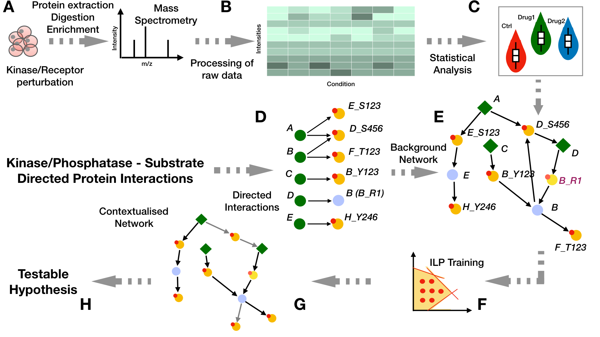
The untargeted phosphoproteomics data (B) used for the identification of the signaling models in PHONEMeS is a data matrix containing the peak heights for each of the measured peptides accross each condition (treatments and control) and replicates and which maps to specific sites over a certain number of proteins (as obtained from the experiments in step A). If the data is not normalized, we quantile normalize the log10 of the raw intensity values and then use a linear model to estimate the effects of each drug over a control state by computing the log fold change between each point of these two conditions and estimating their significance using a t-statistic as computed by the function eBayes implemented by the Bioconductor package limma
As a second step, we fit a Gaussian Mixture Model (GMM) (C) on each peptide accross each condition and select only those peptides whose distributions are better described with 2 components, hence showing a Boolean behaviour under each different condition (perturbed/non-perturbed). For that we can use the Bioconductor package mclust which runs an expectation-maximization method to fit the measurements into mixed Gaussian distributions. Furthermore, we exclude those cases in which the two density curves overlap by more than 10% over a range covering the whole data in order to avoid cases where two conditions are found because of a tightly clustered set of measurements. Then for each point, we associate the score S as the log ratio of the probabilty of belonging to either a control or perturbed state:
\[S_{i,j} = \log 10 (\frac{P_{i,j}(C_i)}{P_{i,j}(P_i)})\]Peptide i is called perturbed under condition j if this score is below the -0.5 value, while for values higher than 0.5 the peptide is considered to be in the control state. Values in between -0.5 and 0.5 are considered as undetermined.
The GMM method can be applied over data which comes from a considerable number of experimental conditions. However data is not usually so sparse. In case we have only a limited number of experimental conditions we can rely on standard differential analysis methods to identify significantly regulated or perturbed sites (C). Users can find examples about how we can generate PHONEMeS inputs with either method here (for GMM) or here (for the differential analysis approach).
From signalling resources such as OmniPath we can assemble a Prior Knowledge Network (PKN) from kinase-to-substrate and directed protein relations (D-E). Green nodes represent proteins that can serve as enzymes. Nodes with small red circles on the top left side represent proteins that can be phosphorylated. Light-blue nodes represent intermediate nodes that can be affected by another protein through other mechanisms besides phosphorylation/dephosphorylation. From the bipartite network representing the enzyme-substrate relationships (D), we obtain the prior knowledge network that is used for the training. This is done as described in (E) by connecting our perturbation targets (diamond green nodes: A, C, and D in this case) with measured phosphosites (yellow nodes with small red circles at the top left) at the protein level and then translating the directed interactions between proteins into their protein-site equivalents. This is achieved by the addition of integrator nodes that propagate the information from a kinase site to the kinase itself (i.e., nodes E, D, and B). This is the network that is used for training. For interactions in which we have no information about the site that is being targeted (i.e., DB), we model it by designating the target node with an auxiliary site that has a recognizable pattern “_R1” (i.e., node B is depicted on the bipartite network as B_R1).
The perturbation signalling network can be inferred (F) by integrating the analysis results obtained from step (B-C) with the PKN we have generated in steps (D-E). This is achieved by the implementation of two optimization methods: 1) Deterministic (PHONEMeS-ILP) and 2) Stochastic (PHONEMeS-stoch).
There are three modes in which we can perform analysis with PHONEMeS-ILP depending on the kind of experimental data we have:
More information about each PHONEMeS-ILP variant can be found on our recent Gjerga et.al. paper.
The previous implementation of PHONEMeS (PHONEMeS-stoch, Terfve et.al.) currently can only handle analysis from perturbation data at single time-point.
Examples about how we can make use of each approach can be found here. After the optimization step, the contextualized network solution are provided as tables which can be visualized through CytoScape (G) and we can further use them to obtain some meaningful biological insights (H).