Tutorial: COSMOS

This tutorial is designed to guide users through the local use of shinyFunky to execute a run of COSMOS. It is highly advised to users to use COSMOS in local session of the shinyFunky app, using the cplex solver.

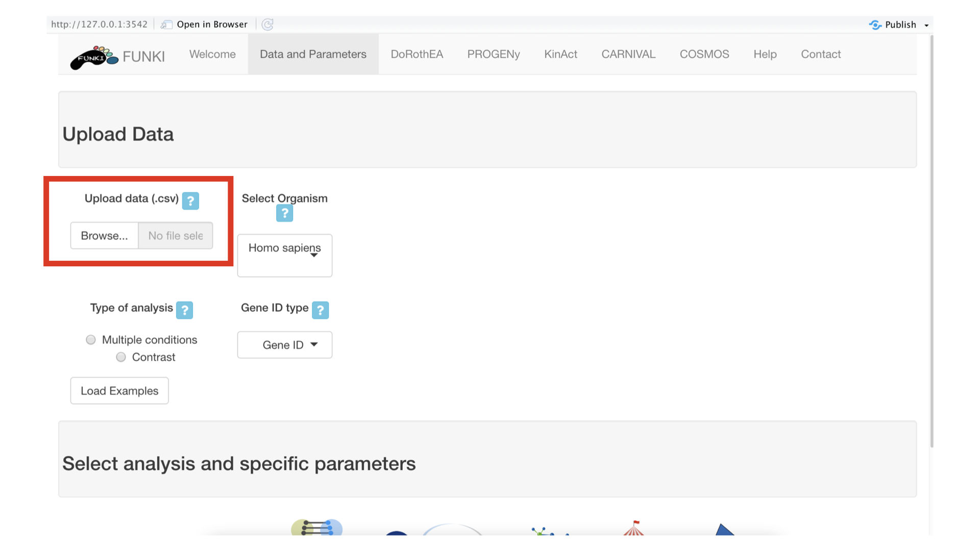
The first step is to upload your gene level differential analysis result (e.i. limma top table output) in which at least one column is named “t” (for t-value), as a csv file. See transcriptutorial for more info on how to obtain normalized counts of differential analysis top table output.

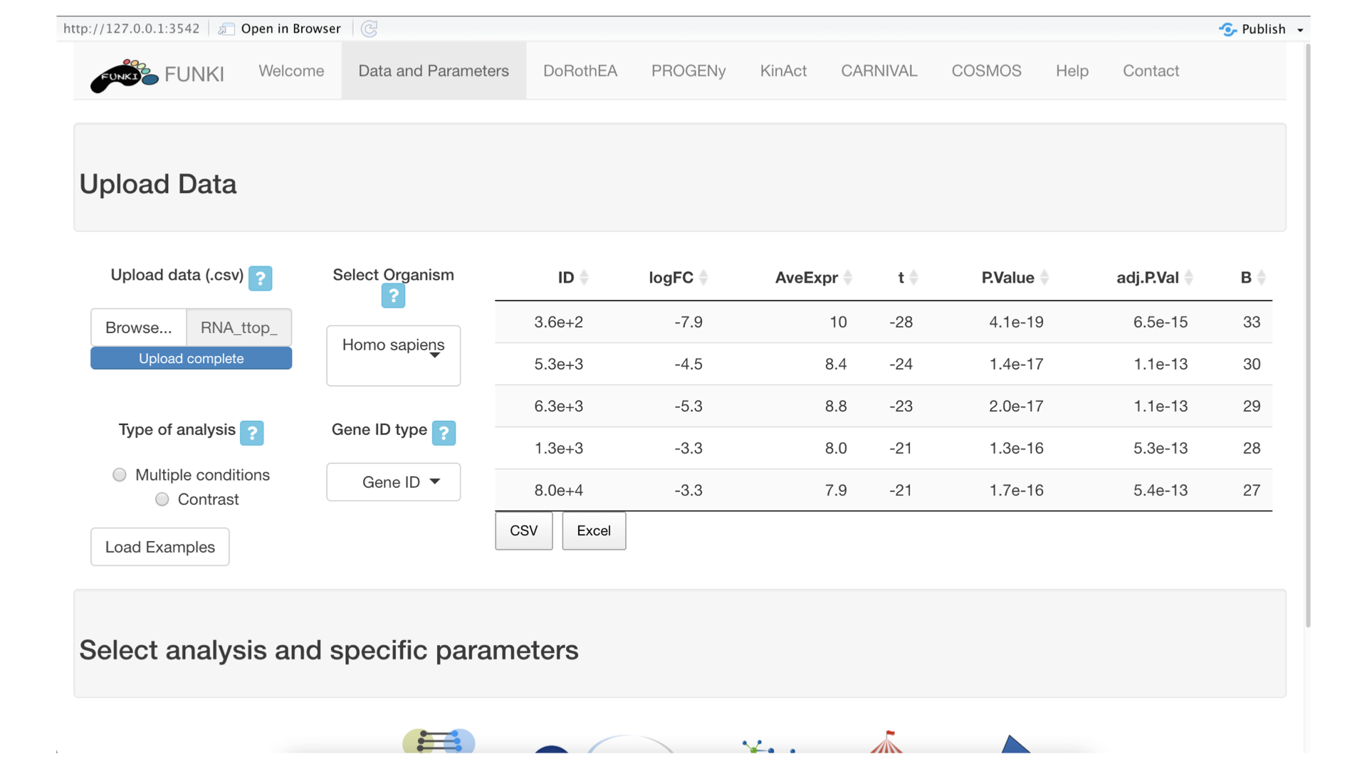
Once the RNA data has been properly uploaded, the table is displayed on the right.

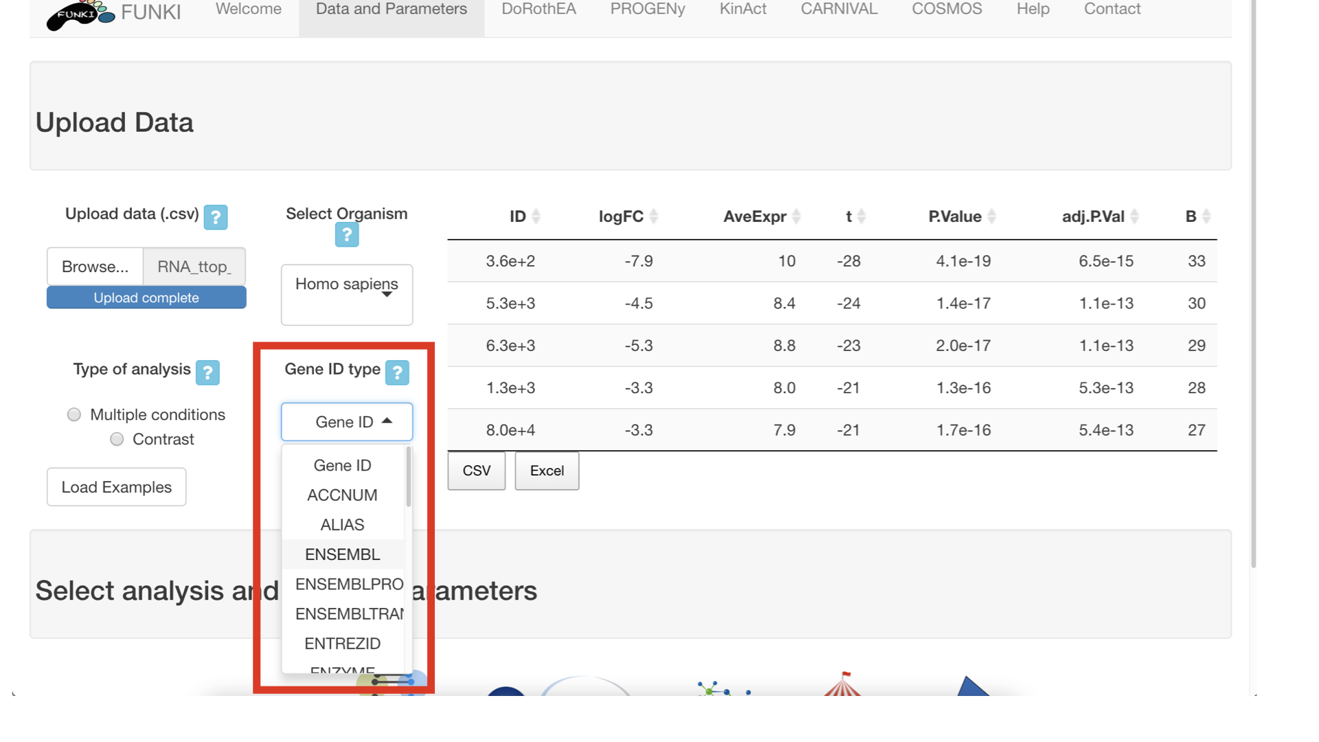
Next, it’s mandatory to indicate what type of identifier is used for the genes. The user can use the drop down list of gene identifiers to indicate the one that corresponds to it’s own data. Entrez gene id are warmly recommended.

Next, go at the bottom of the window and click on the cosmos logo to display the cosmos specific parameters.

You can now upload the data corresponding to the two functional layers that need to be connected together by cosmos. You also need to select which solver to use. At the moment, users are advised to use the IBM cplex solver (free for academics).

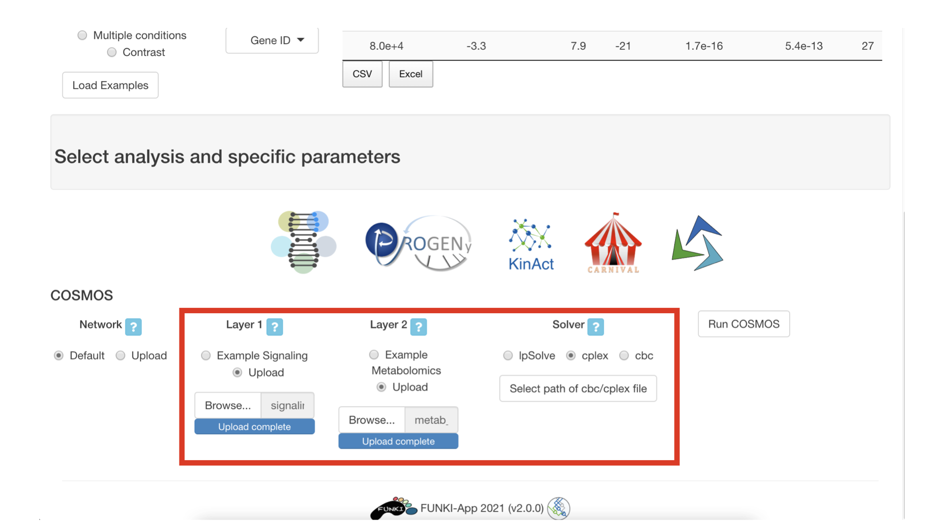
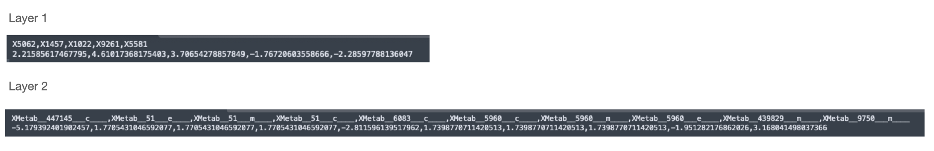
For example, layer 1 can be kinase and TF activities and layer 2 can be metabolic measurements in a csv file, with the first line corresponding to the identifiers and the second line corresponding to measurements. See picture below for what the csv file content should look like.

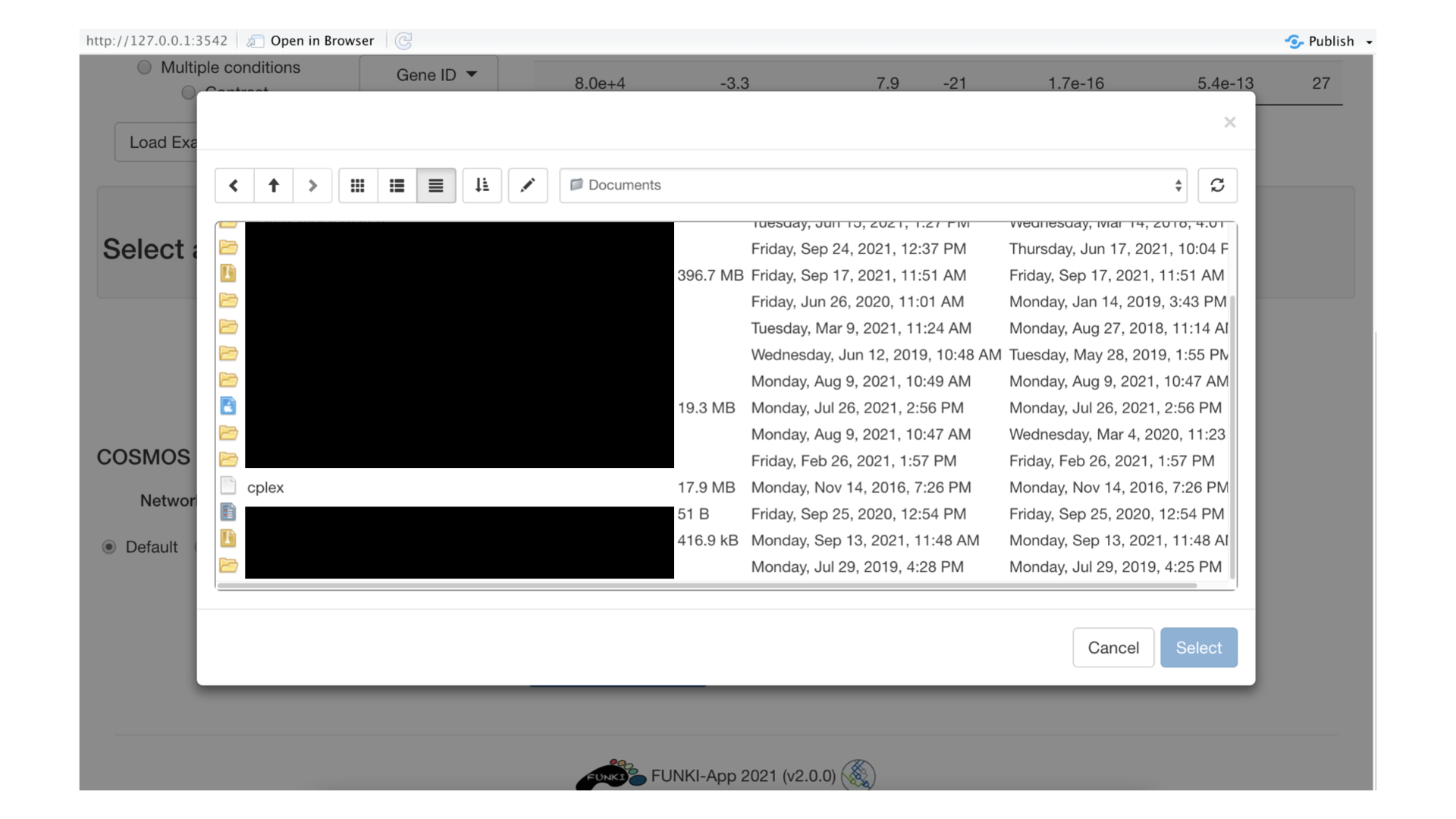
Next, you need to specify the path for the solver executable. For example, The cplex executable is selected in the following picture.

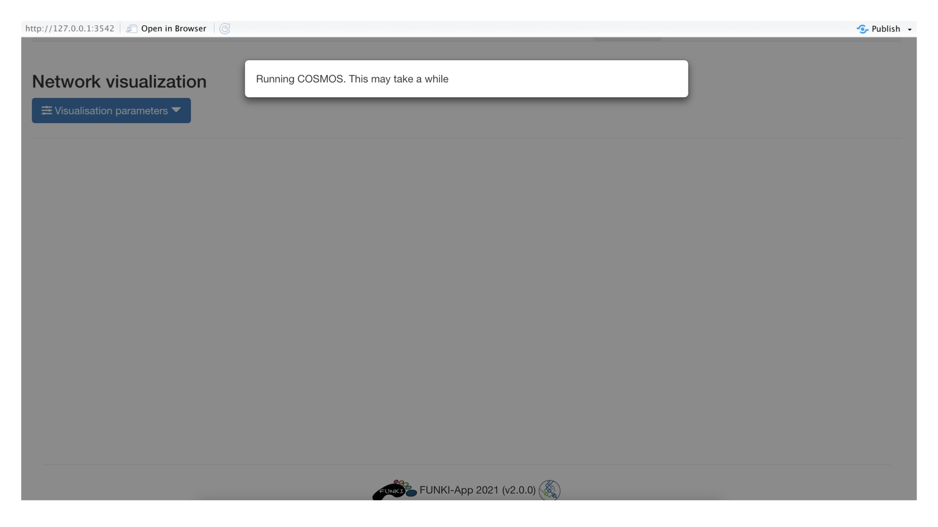
Once everything is set and ready, you can press the “Run COSMOS” button, which should take you to the following screen. Optimizing the network can be a long operation, so you may need to wait a bit (up to 20 or 40 minutes). (You can also follow the progress of the optimisation in the R console).

Once the optimization is done, the resulting network will be displayed. You can click on the “visualization parameters”” button to focus visualization around a specific node or download the result.

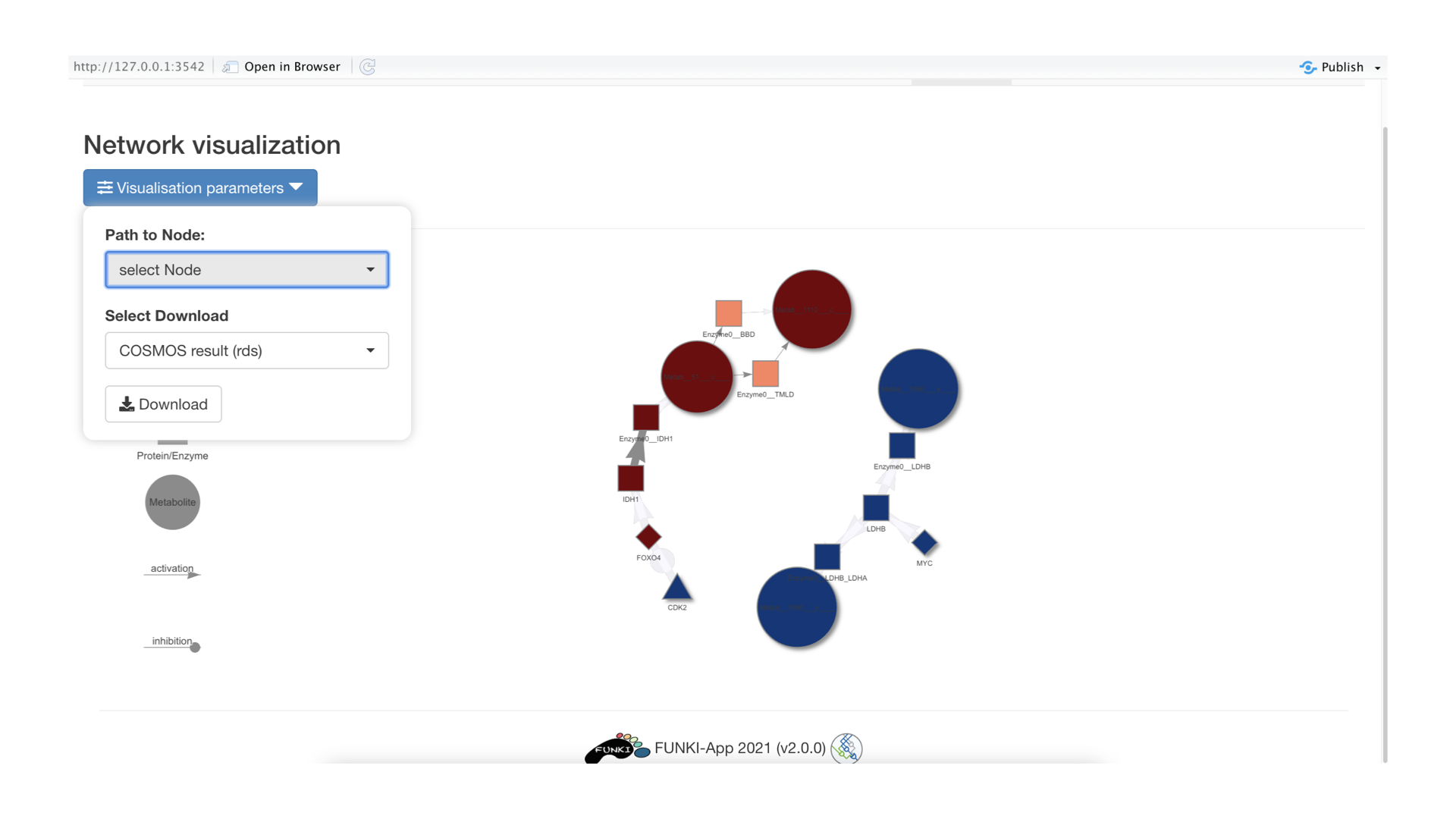
To download the result, you can either download it as an R object (rds) that will contain both the information about the edges and the nodes of the network. If you wish to download the network as csv, you need to download first the file containing the edge information (COSMOS network (csv)) and then the file containing the node attributes (COSMOS attributes (csv)). These files can then be imported in applications like cytoscape to visual the network.