CNODocs contains miscellaneous information that could be useful for users and developers of CellNOpt Software. It is not exhaustive. Other sources of information are contained in the Manuals of each of the packages.
Section author: Thomas Cokelaer
First, load the library:
library(CellNOptR)
First, let us get some data from (cellnopt.data), load it and convert it to a CNOlist data structure, which is the common data structure used in CellNOptR.:
cnolist = CNOlist(CNOdata("MD-ToyMMB.csv"))
Note: The CNOdata function search for the file on the cellnopt.data repository. If not found, it looks on your local directory.
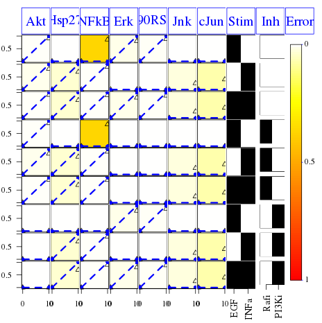
Then, we can look at the content of the cnolist variable using the plotting function:
plot(cnolist)
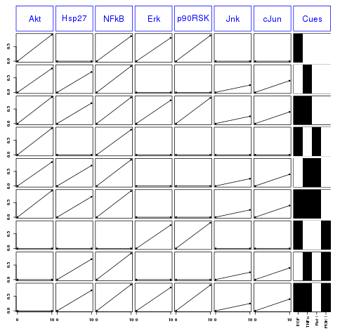
The columns contains each species that has been measured. Each row correspond to different conditions summarized in the last column (cues).
You can get some information about the cnolist variable by printing it:
>>> print(cnolist)
class: CNOlist
cues: EGF TNFa Raf PI3K
inhibitors: Raf PI3K
stimuli: EGF TNFa
timepoints: 0 10
signals: Akt Hsp27 NFkB Erk p90RSK Jnk cJun
variances: Akt Hsp27 NFkB Erk p90RSK Jnk cJun
--
To see the values of any data contained in this instance, just use the
method (e.g., getCues(cnolist), getSignals(cnolist), getVariances(cnolist), ...
And access to one of the field (e.g. signals) by typing:
>>> cnolist@signals
Let us first load a model that should be in SIF format (3 columns CSV like):
library(CellNOptR)
pknmodel = readSIF(CNOdata("PKN-ToyMMB.sif"))
and plot it:
plotModel(pknmodel, output="PNG")
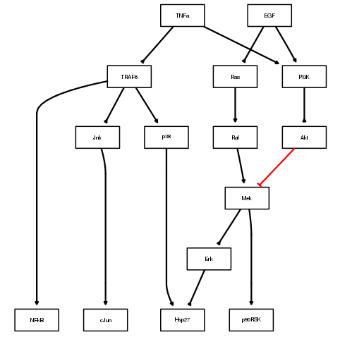
The red edges indicates an inhibitor whereas other black edges are normal links. As we will see in the next section, you can add a cnolist as an argument to colorize this plot.
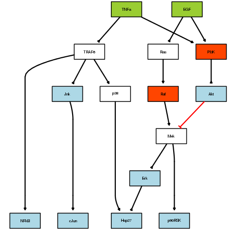
Using the previous CNOlist data structure, you can color the nodes according to their functions:
cnolist = CNOlist(CNOdata("MD-ToyMMB.csv"))
plotModel(pknmodel, cnolist)
Red correspond to inhibitors, green to ligands and blue to measurements.
Let us now optimise a MIDAS data set to a PKN network. First, let us load the data provided within CellNOpt:
library(CellNOptR)              # load the library
data(CNOlistToy, package="CellNOptR")                # load the data
cnolist = CNOlist(CNOlistToy)   # convert to a CNOlist instance
data(ToyModel, package="CellNOptR")                  # load the model
pknmodel = ToyModel             # rename it
You can visualize the Network (with data information) as follows:
plotModel(pknmodel, cnolist)
Preprocess the data before the optimisation:
model = preprocessing(cnolist, pknmodel, compression=TRUE)
Note: The preprocessing performs 3 tasks. First, it removes nodes that are not connected to any cues (green nodes) or readouts (blue nodes). Second, it compresses nodes that are not cues, readouts or inhibitors (red nodes) except those that have multiple inputs AND ouputs (e.g. Mek node in this case). Finally, it expands the nodes that have multiple inputs by adding “and” gates.
As an exercice, you can plot the new processed model.
Now, let us optimise the model against the data with a Genetic Algorithm. There are many optimisation method available in the literature but a GA is good enough for this toy problem. In the following statement with use the gaBinaryT1 function that performs a boolean optimisation on the first time point only:
opt = gaBinaryT1(cnolist, model, verbose=TRUE)
and look at the scores over time:
plotFit(opt)
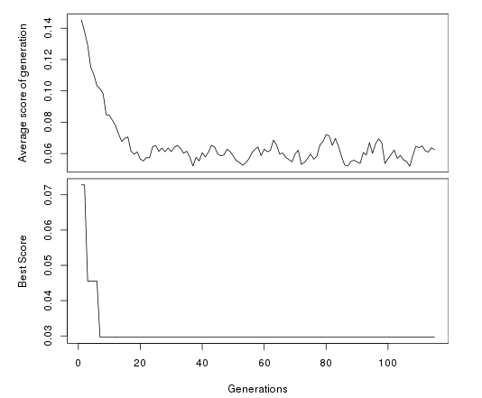
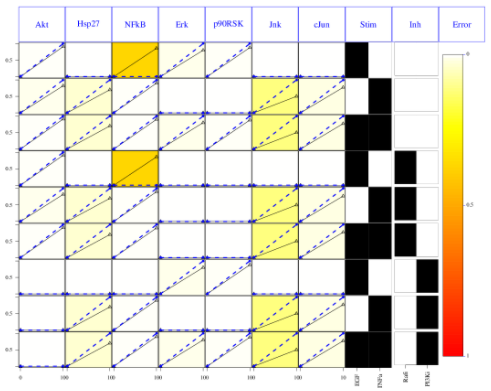
Since it has converged, we can now plot a figure that decomposes the fit of the best model against the data:
cutAndPlot(cnolist, model, bStrings=list(opt$bString))
In the resulting figure we can see that the specy NFkB has a high mismatch, which is indicated by the colored boxes
Finally, we can repeat the previous procedure by including an analysis on a second time point. This can be done with a new set of data that includes 2 time points.
library(CellNOptR)              # load the library
data(CNOlistToy2)
cnolist = CNOlist(CNOlistToy2)
data(ToyModel2, package="CellNOptR")
pknmodel = ToyModel2

# the preprocessing
model = preprocessing(cnolist, pknmodel, compression=TRUE)
optT1 = gaBinaryT1(cnolist, model, verbose=FALSE)
optT2 = gaBinaryTN(cnolist, model, verbose=FALSE, bStrings=list(optT1$bString))
As before, we can look at the first time points results using:
# looking at the results
cutAndPlot(cnolist, model, bStrings=list(optT1$bString))
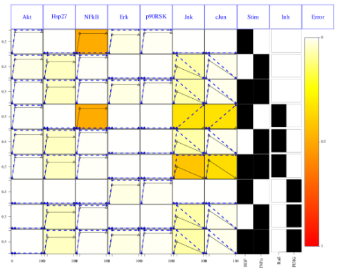
The second optimisation results can be shown using the same function but providing the two optimisation bitstrings:
# looking at the results for 2 time points
cutAndPlot(cnolist, model, bStrings=list(optT1$bString, optT2$bString))
Section author: Thomas Cokelaer, 2013
The SIF format (simple interaction format) is a cytoscape compatible format, which is just a space separated value format. It is convenient for building a graph from a list of interactions. It also makes it easy to combine different interaction sets into a larger network, or add new interactions to an existing data set.
The advantage resides in its simplicity:
specy1 1 specy2
specy1 1 specy3
with the disadvantage that this format does not include any layout information. Each line in a SIF file represent an interaction between a source and one or more target nodes:
nodeA relationship nodeB
nodeC relationship nodeA
nodeD relationship nodeE nodeF nodeB
The SIF format used in CellNOpt is actually a subset of the official SIF format:
#. Generally there is only one target
#. The relationship can be only the number 1 or -1 (for inhibitor)
#. Duplicate entries are not ignored.
Delimiters can be spaces or tabs (mixed).
Duplicated entries are ignored. Multiple edges between the same nodes must have different edge types.
Self loops are also possible:
A 1 A
In cytoscape, the relationship type can be any string. However, in CellNOptR we are limited to the values 1 and -1 that correspond to activation or inhibition.
Section author: Thomas Cokelaer, 2013
This document describes briefly the MIDAS (Minimum Information for Data Analysis in Systems Biology) format that is used in CellNOpt software.
MIDAS files are CSV files (comma separated). The content is defined in the first line of the file that constitutes the header (only 1 line). In the header, colums can take two forms:
XX:Specy,
XX:userword:Specy
where XX is a 2-letter word prefix that describes the column content (see table below for valid word) and Specy is the name of the column. The userword is optional (see later).
MIDAS files include the concept of cues, signals, and responses (Gaudet et al., 2005):
The column headers in a MIDAS files may contain a second (userword) level of identification (e.g. headers for columns describing various cytokine treatments might begin with “TR:Cytokine”). When present, these secondary identifiers allow Software (e.g., DataRail’s importer) to identify automatically the dimensions of a new compendium.
| Code | Description | handled in CellNOptR |
|---|---|---|
| ID | Identifiers | |
| TR | Treatment | yes |
| DA | Data acquisition | yes |
| DV | Data value | yes |
Example:
| TR:mock:CellLine | TR:EGF | TR:TNFa | TR:PI3Ki | DA:Akt | DA:Hsp27 | DV:Akt | DV:Hsp27 |
|---|---|---|---|---|---|---|---|
| 1 | 1 | 0 | 0 | 0 | 0 | 0 | 0 |
| 1 | 0 | 1 | 0 | 0 | 0 | 0 | 0 |
| 1 | 1 | 0 | 0 | 10 | 10 | 1 | 0.2 |
| 1 | 0 | 1 | 0 | 10 | 10 | 1 | 0.5 |
Each value is separated by a comma and you could have space, tabs between commas. So, the final format could be as follows:
TR:mock:CellLine, TR:EGF, TR:TNFa, TR:PI3Ki, DA:Akt, DA:Hsp27, DV:Akt, DV:Hsp27
1,1,0,0, 0,0,   0,0
1,0,1,0, 0,0,   0,0
1,1,0,0, 10,10, 0.82,0.7
1,0,1,0, 10,10, 0.91,0.7
Let us explain the header:
The data above is made of rows that length is as long as the header. Fields may be empty, which is not the case here. If so, software should replace the value by (e.g., NA in R language) and cope with it.
Each row represents a given treatment at a given time. Time are coded with the DA code. Values are coded within the DV columns. Let us look at the 2 first rows. The time is 0. The next two other rows are coded for the time 10. The treatements (3 first colums) are found at the different time.
In MIDAS file, data should be ordered by time although some software may deal with it.
From the Reference below:
MIDAS file has a unique identifier (UID) composed of the following fields:
(i) a two-letter data/file-type code (e.g., PDfor Primary Data, MD for
multiplex data), (ii) a three-letter creator code (typically initials),
(iii) an identification number of arbitrary length that is unique across
the entire system, and (iv) a free-text suffix that serves as a mnemonic
to improve human readability. For example, the primary data discussed in
the text might be tagged MD-LGA-11111-CytoInh17phFI-BLK
In practice, only a few files are coded that way. One reason is that the UID tag is hardly used. Another inconsistency is that dashes are not used or replaced by __. Besides, many files contain the word Data. Finally, the name tag (e.g. LGA above) is not good practice because public file should give the feeling they belong to everybody. However, one consistency is the extension being .csv.
Reference: J. Saez-Rodriguez, A. Goldsipe, J. Muhlich, L. Alexopoulos, B. Millard, D. A. Lauffenburger, P. K. Sorger, Flexible Informatics for Linking Experimental Data to Mathematical Models via DataRail. Bioinformatics, 24:6, 840-847 (2008). Citations
MD-Tag1-Tag2.csv
MD indicates that this is a MIDAS file so no need to set Data in the filename anymore. Tag1 is a general description tag (containing _ possibly) and Tag2 is a variant of Tag1. For instance, Tag1 could be Toy and Tag2 a name to differentiate different Toy data sets.
Correct:
MD-Toy.csv
MD-Toy-variant1.csv
MD-LiverDream.csv
MD-LiverDREAM.csv
There are just a few conventions that should be taken into account when developping/changing CellNOptR and add-on package such as CNORfuzzy, CNORode…
Note: Do not change the layout of a file except if you think it does not fulfill the following conventions.
Correct:
prep4sim
plotFit
readMIDAS
Incorrect:
prep4SIM
PlotFit
readMidas
Some people uses tabs, some others spaces. We decide to use spaces instead of tabs (4 spaces for 1 tab). This is just an arbitrary convention to avoid mixing both without knowing. Easy to set up in any editor.
Code should look like (not the spaces, the curly brackets:
preprocessing <- function(Model){
    m <- Model
    for (r in 1:length(Model$reacID){
        # do something
    } # end of for loop
} # end of main function
At least not something like:
preprocessing <- function(Model){
m <- Model
for (r in 1:length(Model$reacID){
# do something
} # end of for loop
Should follow the same rule as for the naming convention and be consistent over all functions and packages.
Correct:
CNOlist
maxTime
elitism
simList
model
Incorrect:
CNOLIST
MaxTime
Elistism
SimList
Model
Correct:
maxTime, maxtime
simList, simlist
pMutation
Incorrect:
MaxTime
MAXTIME
Pmutation
Ambiguous:
initBstring since B is not a word but an abbreviation. It should be initBitString somehow but this is long. In such case, developer has to make a choice.
You should try to stick to a maximum length of 80 characters per line. Two reasons:
All R functions in the R packages must have a manual that is a file in the man/ directory. The file has the same name as the function that is being documented except for the extension that is .Rd instead of .R
The structure should be as follows:
\name{functionName}
\alias{functionName}
\alias{FUNCTIONNAME}
\title{
    A short description (one line)
}
\description{
    A longer description
}
\usage{
    functionName(arg1, arg2)
}
\arguments{
    \item{arg1}{
        Description of arg1
    }
    \item{arg2}{
        Description of arg2
    }
}
\details{
    Some detailled description
}
\value{
    description of what is returned.
}
\author{
    Your name
}
\seealso{
   \code{\link{anotherFunction}}
    Pointers to related R objects, using \code{\link{...}} to refer to them (\code
    is the correct markup for R object names, and \link produces hyperlinks in
    output formats which support this.
}
\examples{
    data(CNOlistToy,package="CellNOptR")
    data(ToyModel,package="CellNOptR")
    checkSignals(CNOlistToy,ToyModel)

   \dontrun{Some computationally expensive code can be shown but not run.}
   \dontshow{log(x)}    # Only run.
}
\keyword{file}
\note{}
Some fields are optional (e.g., seealso, examples)
The layout is not of importance but to ease the writing/reading of code for developers, please use this layout for the argument section:
\arguments{
    \item{MIDASfile}{
        a CSV MIDAS file (see details)
    }
    \item{verbose}{
        logical (default to TRUE).
    }
}
See the R guidelines
To test if the Rd file is correct, type this command:
R CMD Rd2pdf --vanilla functionName.Rd
If the file is compiled correctly, you should see the PDF is your favorite PDF reader.
Many arguments in CellNOptR and related packages appear often. For instance, CNOlist, Model and so on. Instead of rewriting again and again the text for these arguments, you can use the following convention:
\code{makeCNOlist}\code{readSIF}, normally pre-processed but that is not a requirement of this function\code{indexFinder} from a model.\code{prep4sim}, that has also already been cut to contain only the reactions to be evaluatedIf you use biocLite to install CellNOptR, R dependencies should be installed automatically. However, some libraries may need to be installed by you outside of R.
For example, the Rgraphviz library relies on mesa library.
Under Linux (ubuntu), you should install:
libglu1-mesa-dev
For those insterested to play with the cellnopt.wrapper, which is a Python wrapper, you should install the following librairies:
python-dev
python-rpy2
Under Ubuntu 12.04, during the installation of RCurl package (biocLite(RCurl), I got an error related to a missing rcurl-config.
This can be solved by installing the relevant packages:
sudo apt-get install curl libcurl4-openssl-dev