This documentation is based on the example script (/examples/workflow_preprocessing.R) and data files (data/BxPC3_data.RData” and “data/sampleNames.RData”) provided in the package.
For more detailed information look at the documentation for each funtion (typing “?nameOfFunction” in R).
For this example we will use screening data for the pancreatic cancer cell line BxPC3. Using the microfluidics platform cells were excapsulated in plugs together with drugs (alone or in combination) and a Caspase-3 fluorescent substrate, which becomes green fluorescent when cleaved by active Caspase-3. An automatially controlled Braille Display was used to generate a sequence of 62 experimental condition, each with 12 plugs (20 for the control condition without drugs), which can be considered as replicates. Experiemntal conditions (which will be called samples hereafter) were separated by blue fluorescent plugs used as barcode. An orange fluorescent dye was added to the cell suspension to verify the proper mixture of the components in each plug. Data are recorded using a Labview program developed by R. Utharala which can record three channels (green, blue, orange). During the measurement plugs are flushed at a constant flow rate and are therefore recorded as peaks in the corresponding channels. For more information of the experiment please refer to the paper.
You can load the data provided with the package as follow:
data("BxPC3_data", package="BraDiPluS")
data("sampleNames", package="BraDiPluS")
The first line loads a dataframe called MyData with 4 columns corrisponging to measures in the green, orange and blue channels and acquisition time respectively. The second line loads a vector with corresponding sample names.
MyData includes one full cycle (will be called also run), which is a sequence of the 62 expeirmental conditions mentioned before. Normally the .txt file produced by the Labview program includes more than one sequence of the 62 samples, and these different runs can be separated using the function cutData and specifying start and end time of each run.
To plot the data you can use the following function:
plotData(data=MyData, channels=c("blue", "orange", "green"))
Please check the documentation ?plotData to see additional attributes which can be passed to the function to plot only a specific time range or to highlight info about peaks and samples which can be automatically detected with the functions described in the next sections.
Different samples can be separated based on the peaks in the barcoding channel (which is the blue in our data):
res <- samplesSelection(data=MyData, BCchannel="blue",BCthr=0.01,
	BCminLength=100, distThr=16, plotMyData=T, barcodePos="before")
samples<-res$samples
names(samples)<-sampleNames
Briefly, the samplesSelection function works as follows: 1. detect the barcoding peaks (default blue channel) and that is done considering the blue signal that goes above a defined threshold (set by argument BCthr) and with a minimum width (defined by BCminLength - which unit is number of data points). Then it looks at the space between selected blue peaks and consider as samples those with a distance higher than a threshold (defined by distThr - which unit is time). Arguments shoud be adjusted to properly select the samples. Selected samples can be also plotted using the plotData function.
plotData(data=MyData, channels=c("blue", "orange", "green"), samples = samples)
Samples can then be processed to select the sequence of peaks in the green channel representig the replicates. In this step we can also discart the first peak, to remove potential cross contamination with previous sample, and short peaks, which correspond to unfused plugs.
samplesPeaks <- selectSamplesPeaks(samples, channel="green", metric="median",
	baseThr=0.01, minLength=350, discartPeaks="first", discartPeaksPerc=5)
After these steps, we considered the distribution of the intensity of the orange peaks across all samples and discarded the extreme values (i.e. the outliers). Where Q1 is the 25th percentile, Q3 is the 75th percentile and IQR is the interquantile range (Q3-Q1), outliers were defined as values lower than Q1 - 1.5IQR, or higher than Q3+1.5IQR. Before running the qualityAssessment function, samples with particularly high or low overall orange signal (e.g. due to cells clogging or malfunctioning inlet) were discarded:
samplesPeaks[[indexSampleToRemove]]<-setNames(data.frame(matrix(ncol = ncol(samplesPeaks[[indexSampleToRemove]]), nrow = 0)), colnames(samplesPeaks[[indexSampleToRemove]]))
The function can than be run as:
runs<-list(run1=samplesPeaks)
runs.qa<-qualityAssessment(runs=runs)
If more that one run (i.e. a cycle with all different experimental conditions) is available, and the corresponding peaks are called, for example samplesPeaks1, samplesPeaks2, samplesPeaks3, the function can be called as follows:
runs<-list(run1=samplesPeaks1, run2=samplesPeaks2, run3=samplesPeaks3)
runs.qa<-qualityAssessment(runs=runs)
This part can be run together for all patient/cell line or separately. We will use as example the data provided with the package, that can be load as:
data("allData", package="BraDiPluS")
Data are structured as a list 6 elements, one for each patient/cell line (type names(allData) to check the correspondig names). For example data for cell line BxPC3 can be accessed typing:
BxPC3data <- allData$BxPC3
For each cell line/patient data are also structured as a list with one run (i.e. full repetition of all 62 experimetal conditions) for each element of the list. Each run contains the peaks selected using functions selectSamplesPeaks and qualityAssessment.
For example, we have 2 runs for patient #3 which can be accessed as:
p3data_run1<-allData$patient3$run_1
p3data_run2<-allData$patient3$run_2
All runs for all patient/cell lines must have the same number of elements (which should correspond to the total number of experimental conditions, 62 in our case).
The function can be applied to all patient/cell lines as follows:
res<-computeStatistics(allData, controlName="FS + FS", thPval=0.1, thSD=1.5, subsample=F, saveFiles=T)
Here below we will consider patient #3 to illustrate the usage of function computeStatistics.
exampleData <- list(patient2=allData$patient2)
setwd("path/to/fuguresFolder")
res<-computeStatistics(exampleData, controlName="FS + FS", thPval=0.1, thSD=1.5, subsample=F, saveFiles=T)
This will produce two figures called “boxplot.pdf” and “volcanoplot.pdf” and outputs a data.frame with the computed zscores and p-values for each sample and each patient/cell line, along with info about which samples are significant based on the used defined criteria. For each patient/cell line the z-score is computed separately for each run and then averaged. P-values are also computed separately for each run, using Wilcoxon rank sum test to verify if the response to the tested drugs (alone or in combination) is significantly higher than the measurements for control condition (no perturbation). P-values were FDR-corrected for multiple hypotheses testing and combined across different runs using Fisher’s method. Optionally a threshold on the standard deviation (SD) of the distribution of the z-score for each sample can also be set, to further limit the analysis to samples with low variability across runs.
The resulting boxplot for patient #3 is:
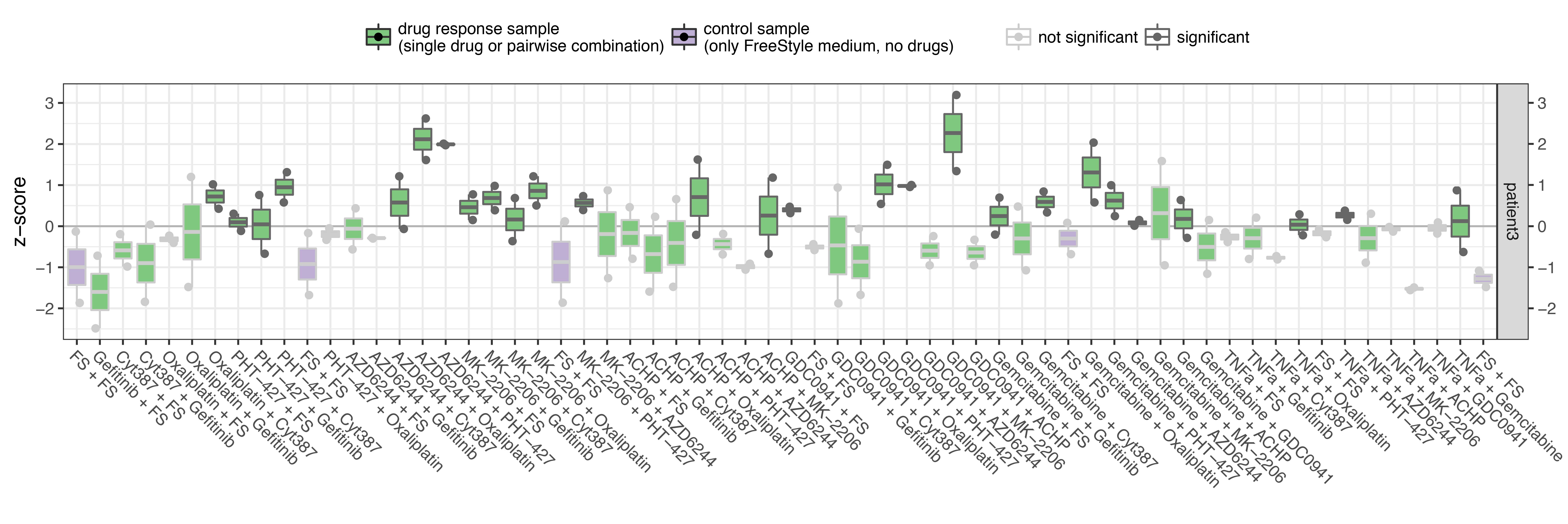
For each of the 62 samples the z-score for each run is plotted as a dot (we have 2 runs in this case, resulting in 2 dots for each sample) and the distribution of the z-scores across runs is shown as a boxplot for each sample (more meaningful when more than 2 runs available). The boxplots are coloured in green for perturbed conditions and in purple for the control (unperturbed) samples to visually assess if control samples are reasonably constant over time. Samples are considered significant when p-val < thPval and and SD < thSD (if thSD is defined, otherwise only thresold on p-value is considered).
The resulting volcano plot for patient #3 is:
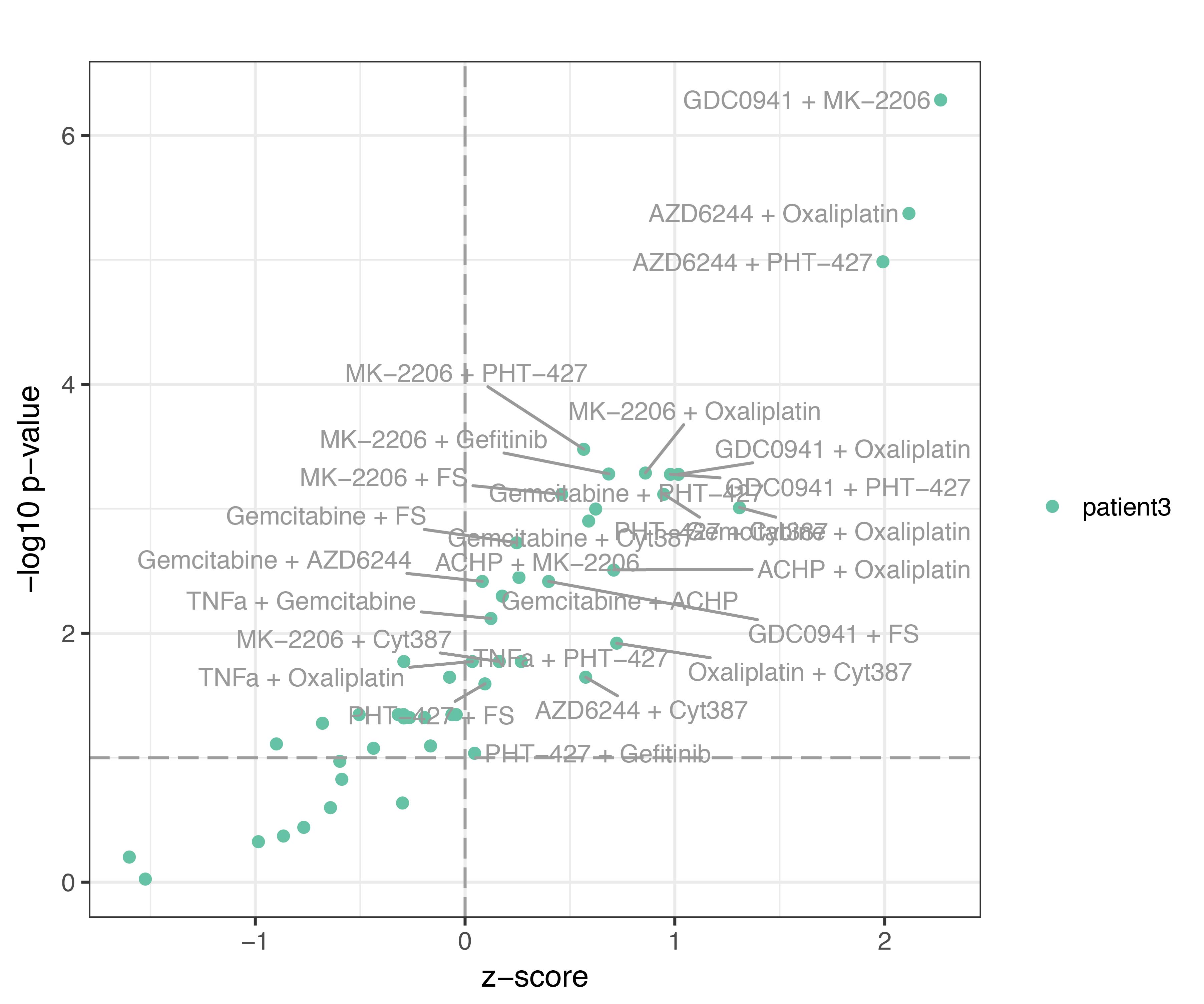
The z-score (avereage across runs) is plotted versus the -log10 of the p-value for the 62 samples (dots). In this case, all samples with z-score > 0 are also significantly different from the control condition.