browse_results
Jovan Tanevski
2022-01-25
Last updated: 2022-01-25
Checks: 7 0
Knit directory: mistyMBC/
This reproducible R Markdown analysis was created with workflowr (version 1.7.0). The Checks tab describes the reproducibility checks that were applied when the results were created. The Past versions tab lists the development history.
Great! Since the R Markdown file has been committed to the Git repository, you know the exact version of the code that produced these results.
Great job! The global environment was empty. Objects defined in the global environment can affect the analysis in your R Markdown file in unknown ways. For reproduciblity it’s best to always run the code in an empty environment.
The command set.seed(42) was run prior to running the
code in the R Markdown file. Setting a seed ensures that any results
that rely on randomness, e.g. subsampling or permutations, are
reproducible.
Great job! Recording the operating system, R version, and package versions is critical for reproducibility.
Nice! There were no cached chunks for this analysis, so you can be confident that you successfully produced the results during this run.
Great job! Using relative paths to the files within your workflowr project makes it easier to run your code on other machines.
Great! You are using Git for version control. Tracking code development and connecting the code version to the results is critical for reproducibility.
The results in this page were generated with repository version eade820. See the Past versions tab to see a history of the changes made to the R Markdown and HTML files.
Note that you need to be careful to ensure that all relevant files for
the analysis have been committed to Git prior to generating the results
(you can use wflow_publish or
wflow_git_commit). workflowr only checks the R Markdown
file, but you know if there are other scripts or data files that it
depends on. Below is the status of the Git repository when the results
were generated:
Ignored files:
    Ignored:    .DS_Store
    Ignored:    .Rhistory
    Ignored:    .Rproj.user/
    Ignored:    analysis/.DS_Store
    Ignored:    code/
    Ignored:    data/
    Ignored:    omnipathr-log/
    Ignored:    output/.DS_Store
    Ignored:    output/HTAPP-213-SMP-6752/.DS_Store
    Ignored:    output/HTAPP-213-SMP-6752/HTAPP-213-SMP-6752_slide_seq_processed-1/.DS_Store
    Ignored:    output/HTAPP-364-SMP-1321/.DS_Store
    Ignored:    output/HTAPP-364-SMP-1321/HTAPP-364-SMP-1321_codex_processed-1_failed/
    Ignored:    output/HTAPP-364-SMP-1321/HTAPP-364-SMP-1321_slide_seq_processed-2/.DS_Store
Note that any generated files, e.g. HTML, png, CSS, etc., are not included in this status report because it is ok for generated content to have uncommitted changes.
These are the previous versions of the repository in which changes were
made to the R Markdown (analysis/browse_results.Rmd) and
HTML (docs/browse_results.html) files. If you’ve configured
a remote Git repository (see ?wflow_git_remote), click on
the hyperlinks in the table below to view the files as they were in that
past version.
| File | Version | Author | Date | Message |
|---|---|---|---|---|
| Rmd | eade820 | Jovan Tanevski | 2022-01-25 | wflow_publish("analysis/browse_results.Rmd") |
| Rmd | 48a8a6c | Jovan Tanevski | 2022-01-25 | liver contrasts |
| html | ec6405d | Jovan Tanevski | 2021-10-29 | Build site. |
| Rmd | 4abf508 | Jovan Tanevski | 2021-10-29 | update result browsing to match new parameters |
| html | cb33a3e | Jovan Tanevski | 2021-09-23 | Build site. |
| Rmd | 02a4d8f | Jovan Tanevski | 2021-09-23 | add metadata and signature pca |
| html | 6a3c444 | Jovan Tanevski | 2021-09-15 | Build site. |
| Rmd | c6d135a | Jovan Tanevski | 2021-09-15 | extend results with celltype analysis |
| html | 6398d1c | Jovan Tanevski | 2021-09-13 | Build site. |
| Rmd | b562161 | Jovan Tanevski | 2021-09-13 | merge codex and merfish results |
| html | c457348 | Jovan Tanevski | 2021-09-09 | Build site. |
| html | aa6ca6b | Jovan Tanevski | 2021-09-09 | Build site. |
| Rmd | 04b30ad | Jovan Tanevski | 2021-09-09 | clean up results, focus on targets with gain |
| html | 2438eb2 | Jovan Tanevski | 2021-09-09 | Build site. |
| Rmd | b124494 | Jovan Tanevski | 2021-09-09 | update codex,merfish; add slideseq cellcom results |
| html | e0c1952 | Jovan Tanevski | 2021-07-22 | Build site. |
| html | 4dd6a02 | Jovan Tanevski | 2021-07-14 | Build site. |
| html | 913535e | Jovan Tanevski | 2021-06-17 | Build site. |
| Rmd | 736d8e3 | Jovan Tanevski | 2021-06-17 | subset merfish results |
| html | 1b68c27 | Jovan Tanevski | 2021-06-15 | Build site. |
| Rmd | 43913a8 | Jovan Tanevski | 2021-06-15 | auto publish date |
| Rmd | 34b1d9e | Jovan Tanevski | 2021-06-15 | explicit codex, merfish and exseq |
| html | e445e6f | Jovan Tanevski | 2021-06-11 | Build site. |
| Rmd | dd0219f | Jovan Tanevski | 2021-06-11 | add result browsing example |
Setup
Load necessary libraries
library(stringr)
library(dplyr)
library(readr)
library(mistyR)
library(ggplot2)
library(future)
library(factoextra)

plan(multisession)
Output collection
Find the location of the results for all samples
outputs <- str_subset(list.dirs("output"), "processed") %>%
  str_subset("failed", negate = TRUE) %>%
  str_subset("slide_seq_processed-[0-9]$", negate = TRUE)
Collect the results for all samples, single modality and all replicates
misty.results.codex <- collect_results(str_subset(outputs, "codex"))
Collecting improvements
Collecting contributions
Collecting importances
Aggregatingmisty.results.merfish <- collect_results(str_subset(outputs, "merfish"))
Collecting improvements
Collecting contributions
Collecting importances
Aggregatingmisty.results.ligrcp <- collect_results(str_subset(outputs, "ligrcp"))
Collecting improvements
Collecting contributions
Collecting importances
Aggregatingmisty.results.ligpath <- collect_results(str_subset(outputs, "ligpath"))
Collecting improvements
Collecting contributions
Collecting importances
AggregatingGet metadata
sample.meta <- read.delim("data/HTAPP_MBC_spatial_annotations.tsv",
  na.strings = ""
)
Plot basic results
CODEX
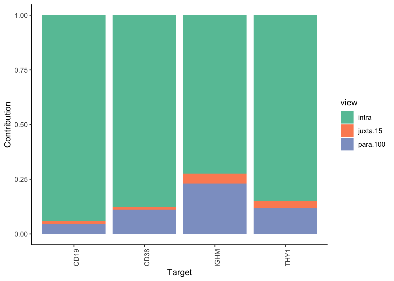
Filter only genes with mean gain in variance explained of .5% or more to plot the gain and view contributions
misty.results.codex %>%
  plot_improvement_stats(trim = 0.5) %>%
  plot_view_contributions(trim = 0.5)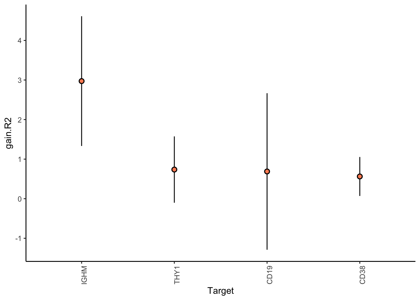
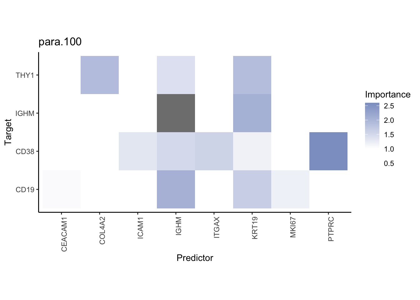
Plot interaction heatmaps
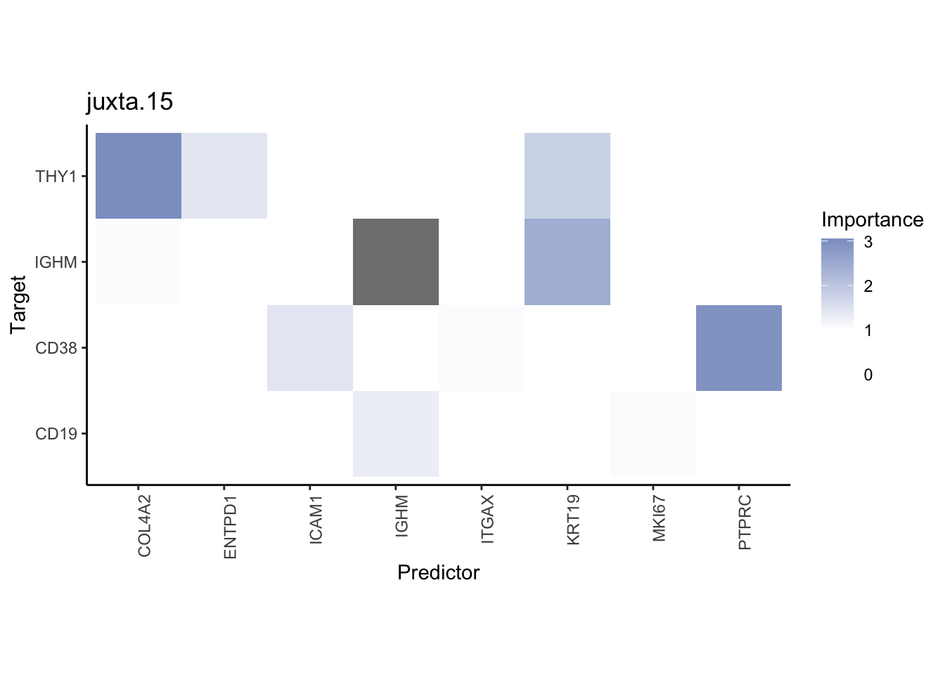
misty.results.codex %>%
  plot_interaction_heatmap("intra", cutoff = 4, clean = TRUE) %>%
  plot_interaction_heatmap("juxta.15", cutoff = 1, clean = TRUE, trim = 0.5) %>%
  plot_interaction_heatmap("para.100", cutoff = 1, clean = TRUE, trim = 0.5)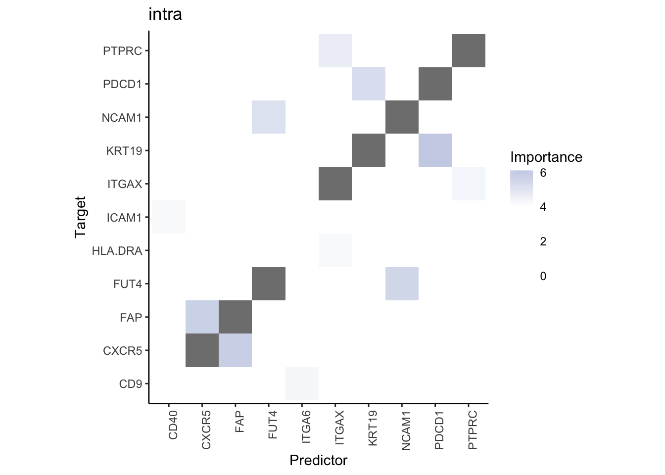
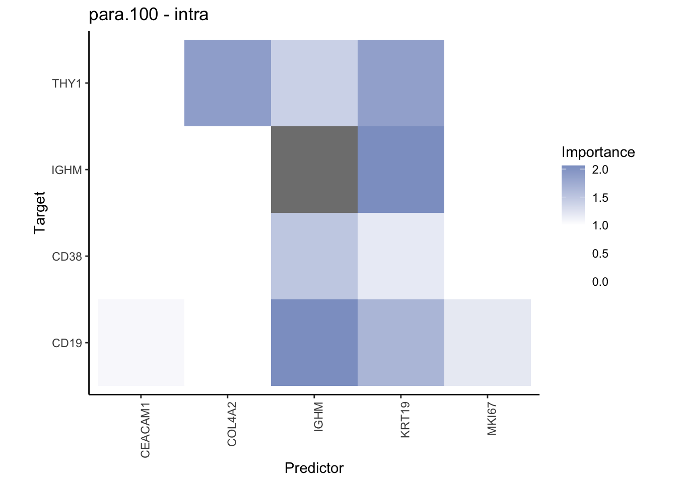
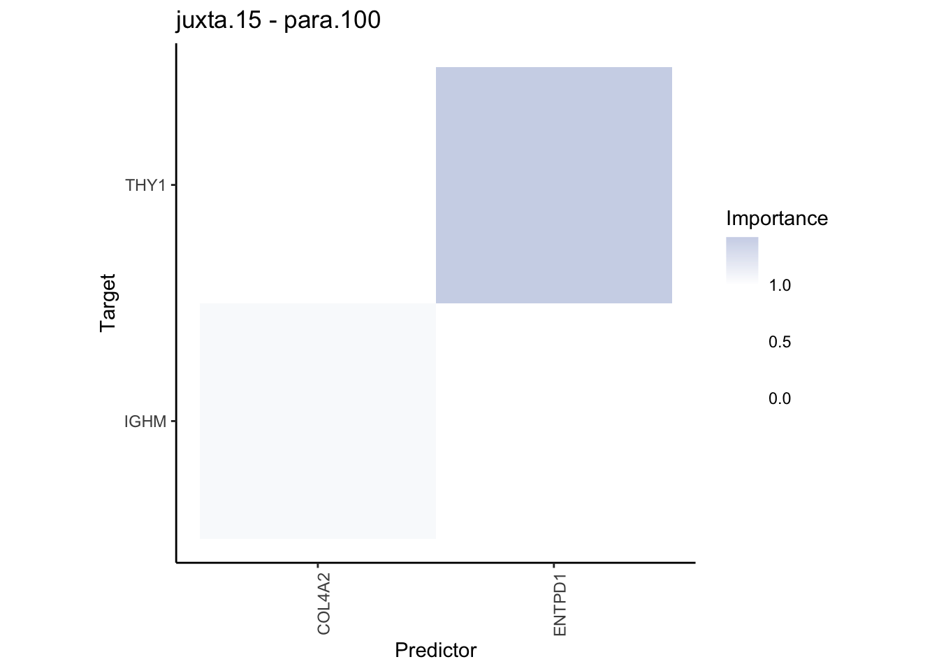
Plot contrasts
misty.results.codex %>%
  plot_contrast_heatmap("intra", "juxta.15", cutoff = 1, trim = 0.5) %>%
  plot_contrast_heatmap("intra", "para.100", cutoff = 1, trim = 0.5) %>%
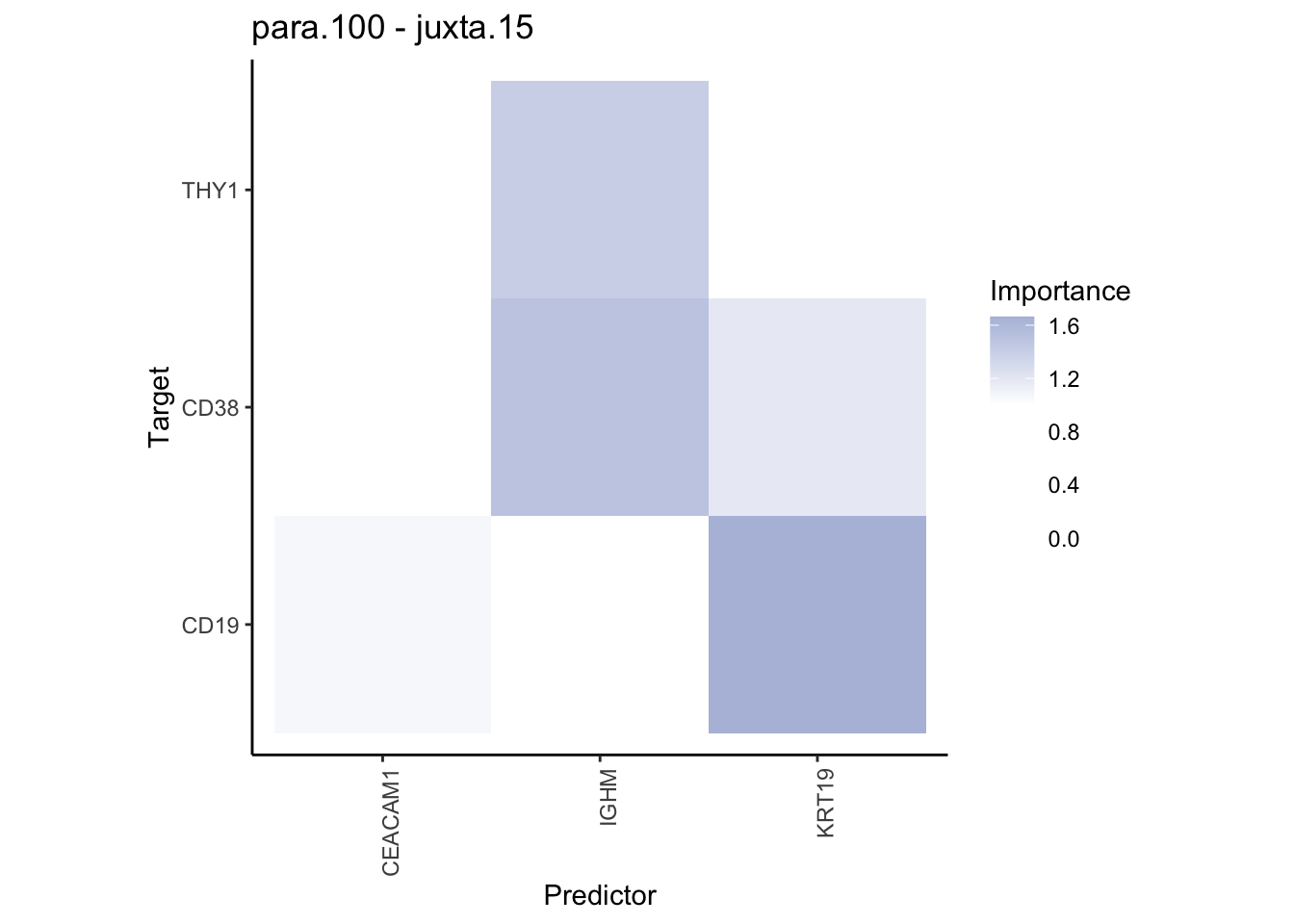
  plot_contrast_heatmap("para.100", "juxta.15", cutoff = 1, trim = 0.5) %>%
  plot_contrast_heatmap("juxta.15", "para.100", cutoff = 1, trim = 0.5)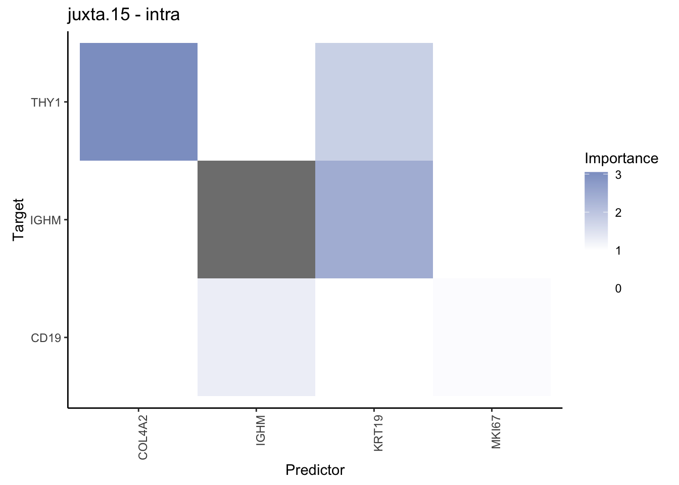
| Version | Author | Date |
|---|---|---|
| ec6405d | Jovan Tanevski | 2021-10-29 |
Plot interaction communities
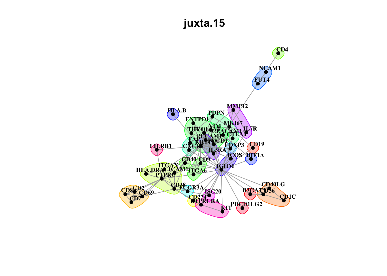
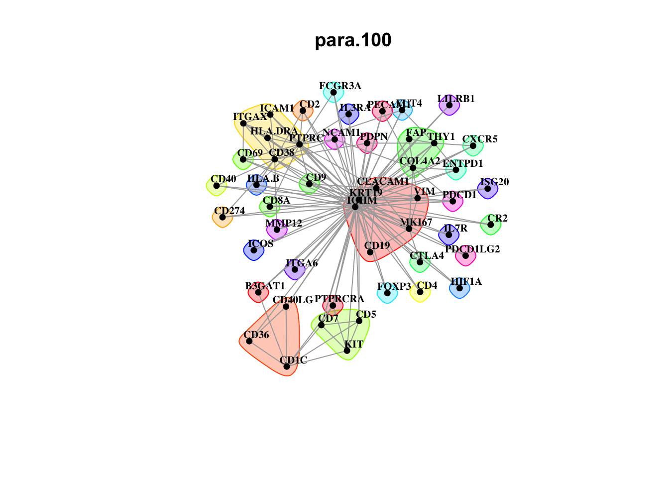
misty.results.codex %>%
  plot_interaction_communities("intra", cutoff = 4) %>%
  plot_interaction_communities("juxta.15", cutoff = 1) %>%
  plot_interaction_communities("para.100", cutoff = 1)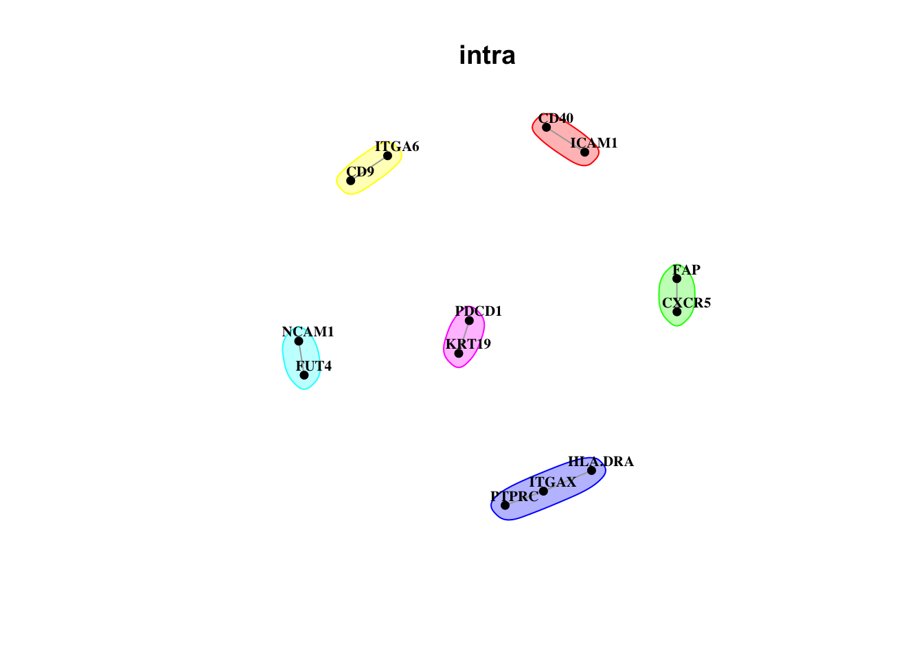
Signatures and clustering
signature.per.codex <- misty.results.codex %>%
  extract_signature("performance", trim = 0.5) %>%
  mutate(sample = str_extract(sample, "HTAPP(-[:alnum:]+){3}"))

signature.per.pca <- signature.per.codex %>%
  select(-sample) %>%
  prcomp()

signature.per.pca.ann <- left_join(bind_cols(
  signature.per.codex %>% select(sample),
  as.data.frame(signature.per.pca$x)
),
sample.meta,
by = c("sample" = "name")
)


ggplot(signature.per.pca.ann, aes(x = PC1, y = PC2)) +
  geom_point(aes(color = site_biopsy)) +
  theme_classic()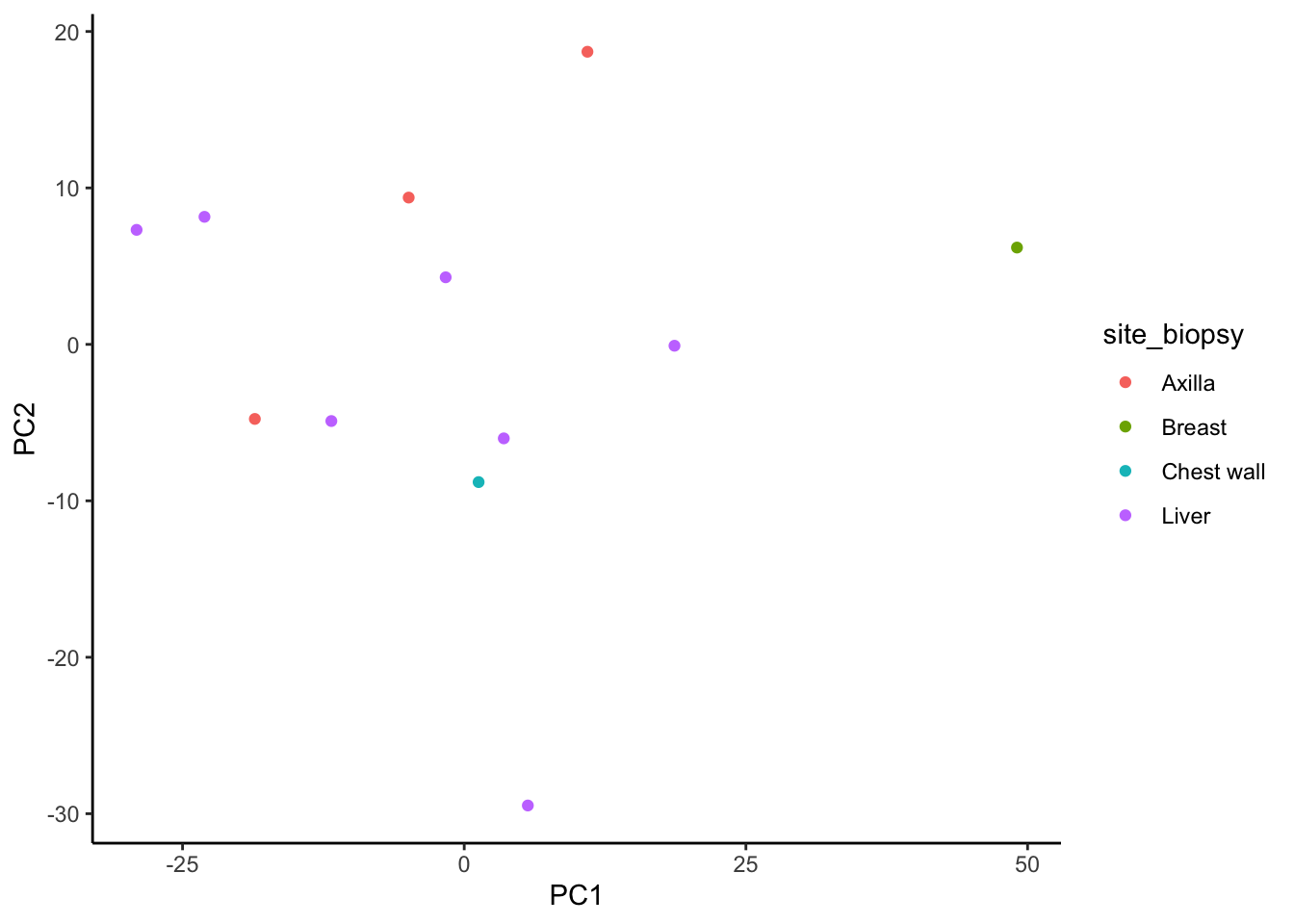
ggplot(signature.per.pca.ann, aes(x = PC1, y = PC2)) +
  geom_point(aes(color = receptors_biopsy)) +
  theme_classic()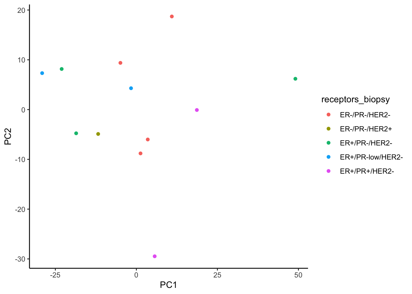
fviz_pca_var(signature.per.pca, col.var = "cos2", gradient.cols = c("#666666", "#377EB8", "#E41A1C"), repel = TRUE) + theme_classic()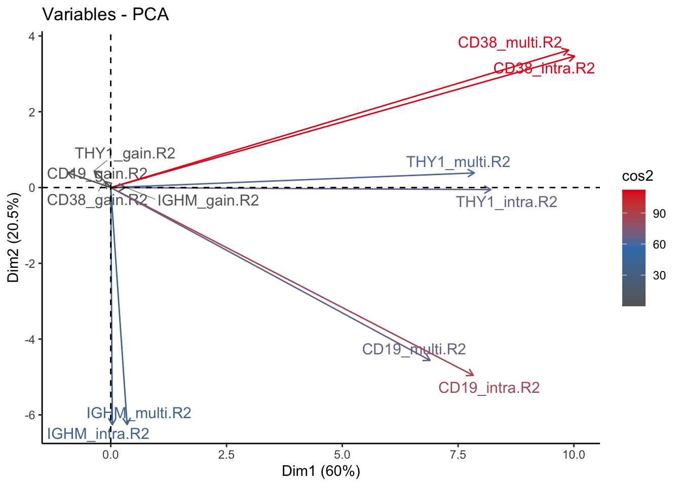
Compare samples from liver biopsies to all other
codex.liver <- str_subset(outputs, "codex") %>%
  str_subset(sample.meta %>%
               filter(site_biopsy == "Liver") %>%
               pull(name) %>%
               str_extract("\\d+$") %>%
               paste0(.,collapse = "|"))

codex.other <- str_subset(outputs, "codex") %>%
  str_subset(sample.meta %>%
               filter(site_biopsy != "Liver") %>%
               pull(name) %>%
               str_extract("\\d+$") %>%
               paste0(.,collapse = "|"))

results.codex.liver <- collect_results(codex.liver)
Collecting improvements
Collecting contributions
Collecting importances
Aggregatingresults.codex.other <- collect_results(codex.other)
Collecting improvements
Collecting contributions
Collecting importances
Aggregatingresults.codex.liver %>% plot_improvement_stats(trim = 0.5)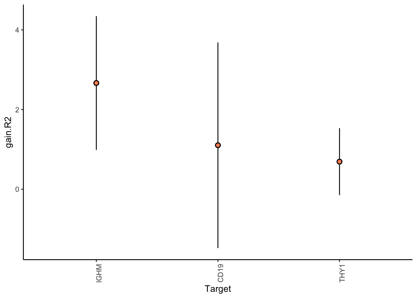
results.codex.other %>% plot_improvement_stats(trim = 0.5)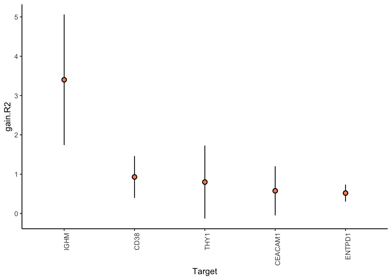
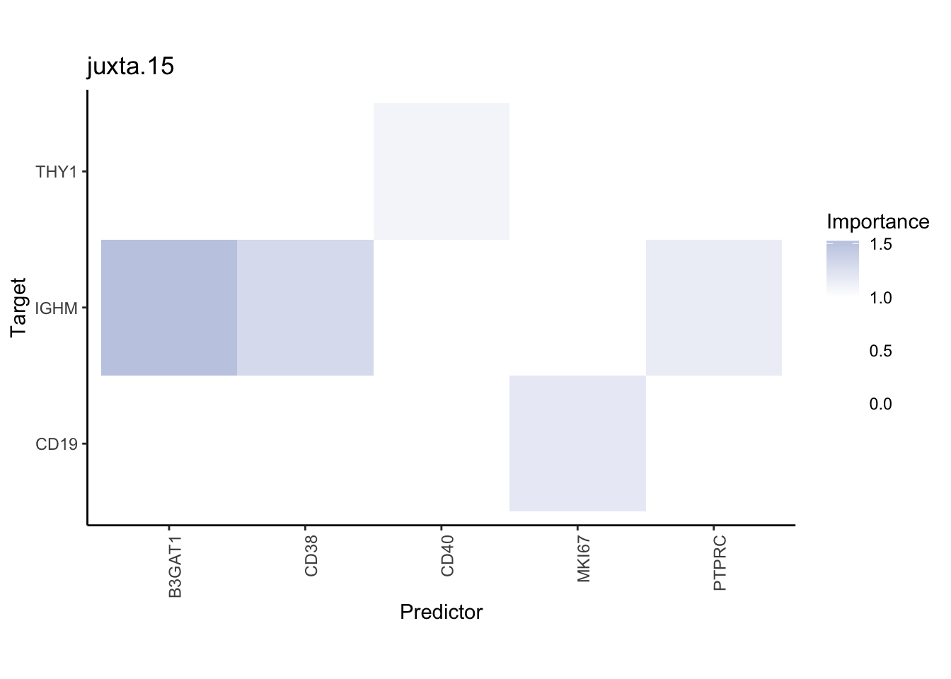
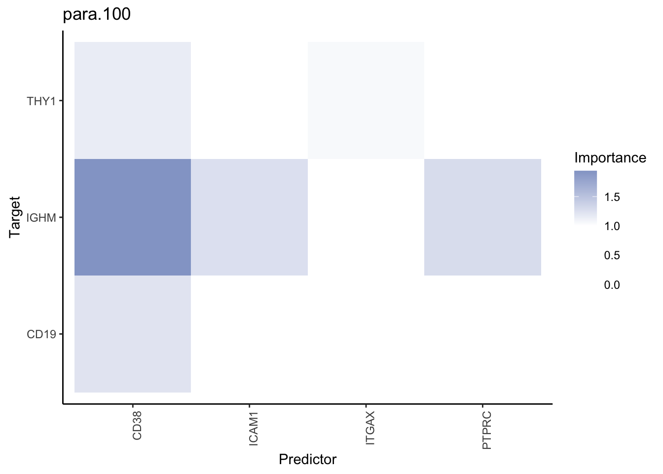
Liver specific interactions
plot_contrast_results(results.codex.liver, results.codex.other, trim = 0.5)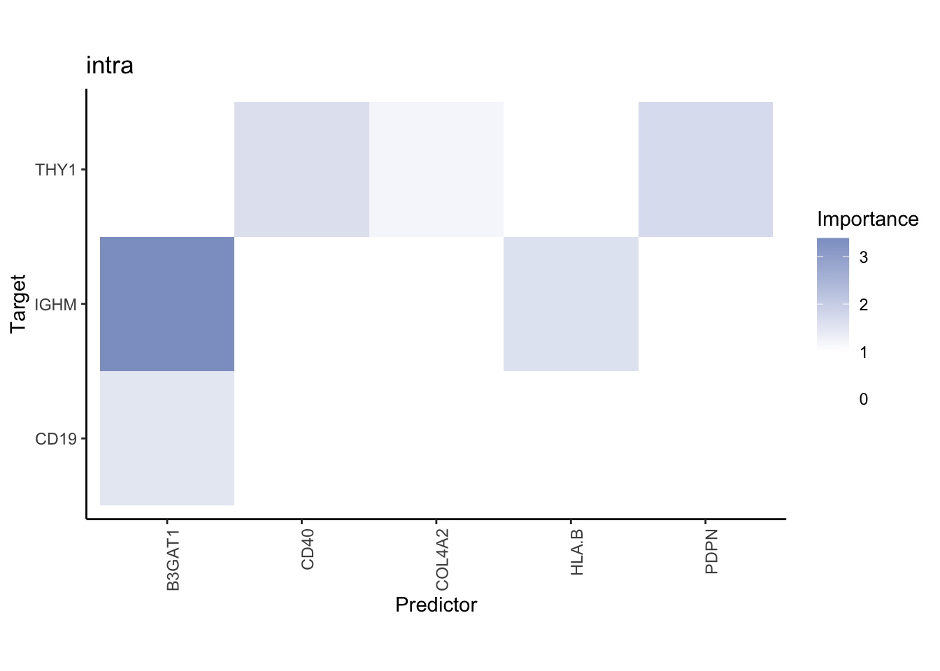
MERFISH
We combine the information from binned and unbinned samples.
Filter only genes with mean gain in variance explained of 2 or more to plot the gain and view contributions
MERFISH shows much better performance improvement than CODEX, but captures much less information in the intraview on average.
misty.results.merfish %>%
  plot_improvement_stats(trim = 2) %>%
  plot_view_contributions(trim = 2)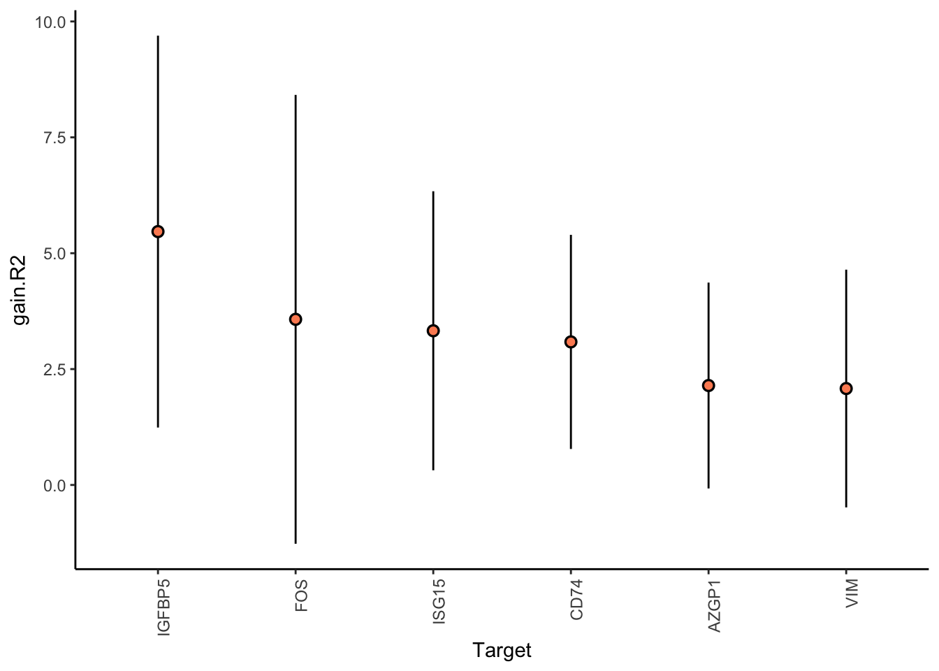
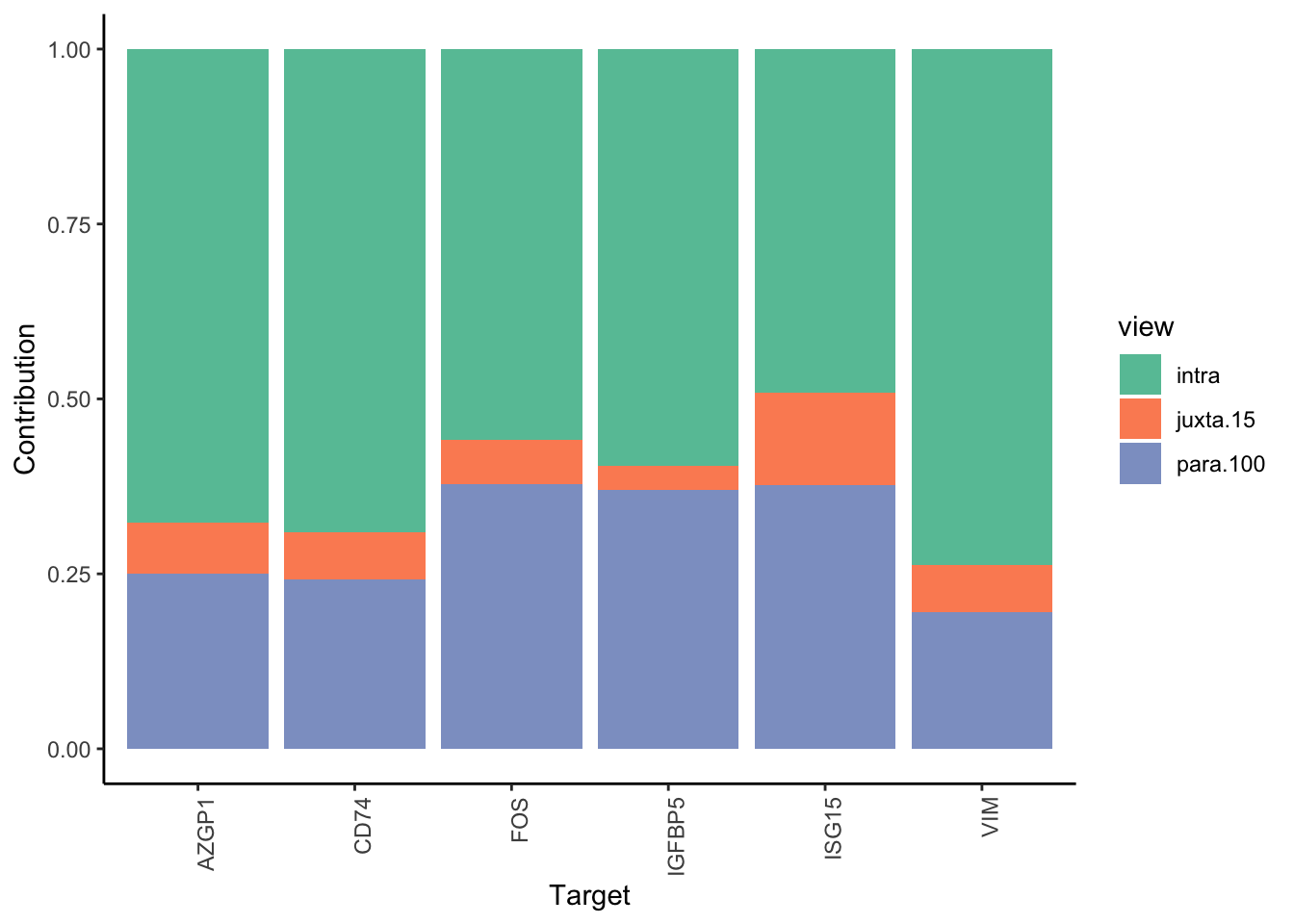
MERFISH shows much better performance improvement than CODEX, but captures much less information in the intraview on average.
misty.results.merfish$improvements %>%
  filter(measure == "intra.R2") %>%
  pull(value) %>%
  hist(main = "MERFISH distribution of variance explained in intraview")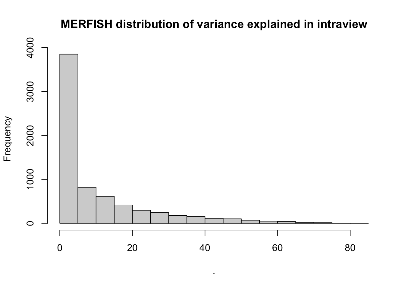
misty.results.merfish$improvements %>%
  filter(measure == "gain.R2") %>%
  pull(value) %>%
  hist(main = "MERFISH distribution of gain in variance explained")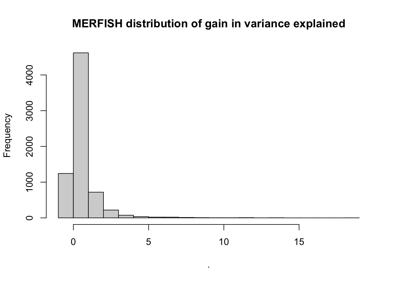
misty.results.codex$improvements %>%
  filter(measure == "intra.R2") %>%
  pull(value) %>%
  hist(main = "CODEX distribution of variance explained in intraview")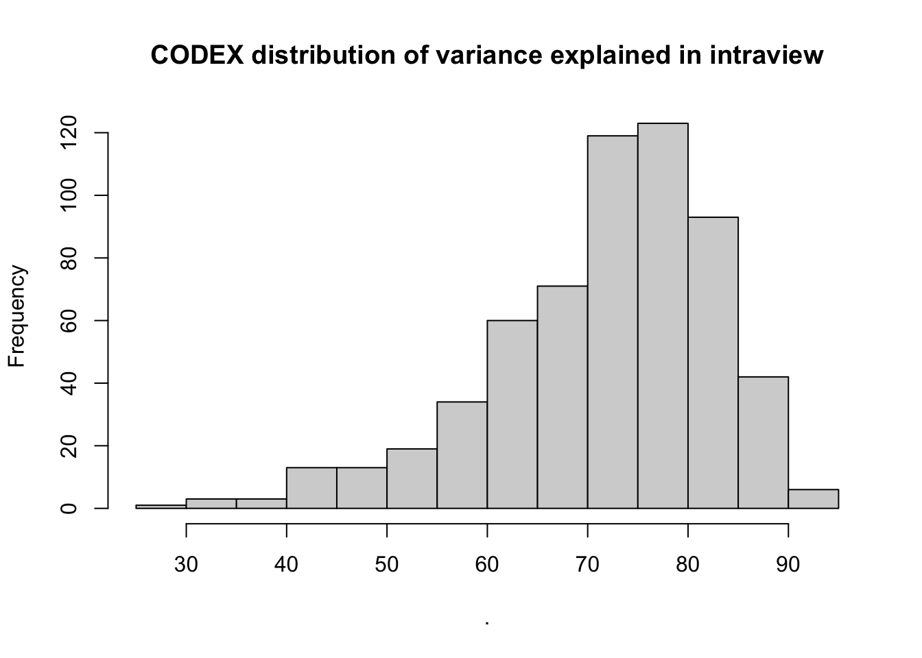
misty.results.codex$improvements %>%
  filter(measure == "gain.R2") %>%
  pull(value) %>%
  hist(main = "CODEX distribution of gain in variance explained")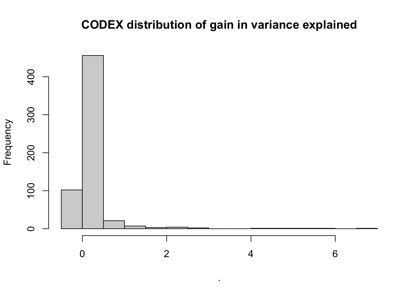
| Version | Author | Date |
|---|---|---|
| ec6405d | Jovan Tanevski | 2021-10-29 |
Plot interaction heatmaps
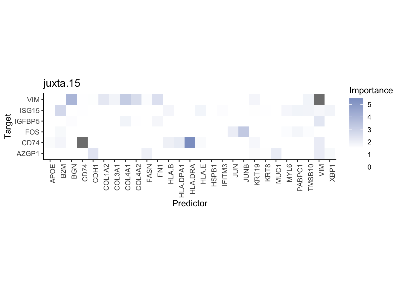
misty.results.merfish %>%
  plot_interaction_heatmap("intra", cutoff = 6, clean = TRUE) %>%
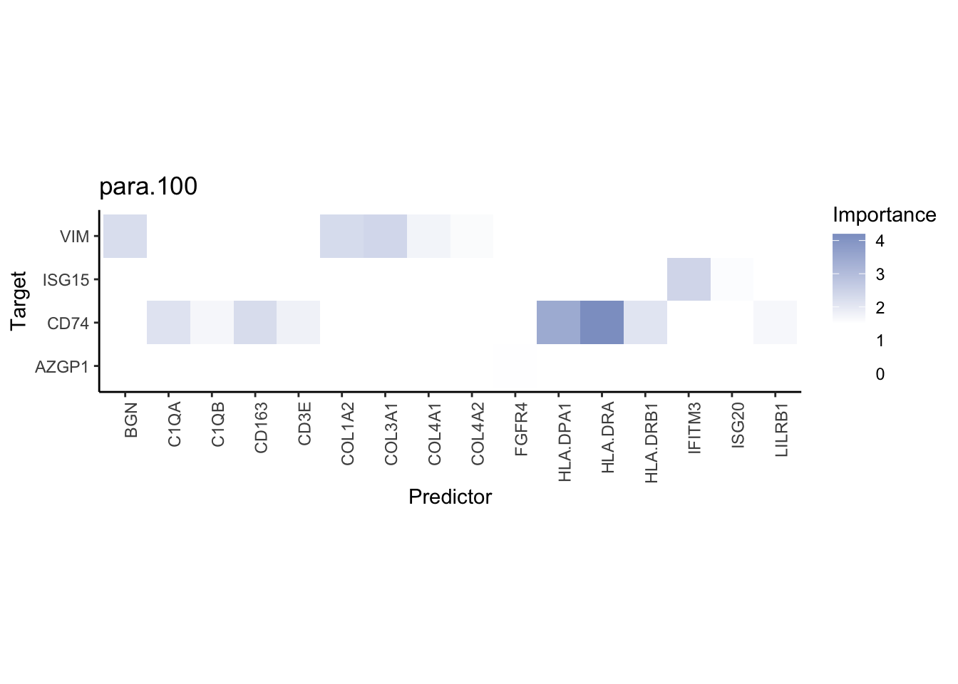
  plot_interaction_heatmap("juxta.15", cutoff = 1.5, clean = TRUE, trim = 2) %>%
  plot_interaction_heatmap("para.100", cutoff = 1.5, clean = TRUE, trim = 2)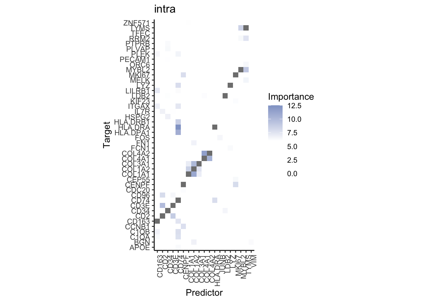
Plot contrasts
misty.results.merfish %>%
  plot_contrast_heatmap("intra", "juxta.15", cutoff = 1.5, trim = 2) %>%
  plot_contrast_heatmap("intra", "para.100", cutoff = 1.5, trim = 2) %>%
  plot_contrast_heatmap("para.100", "juxta.15", cutoff = 1.5, trim = 2) %>%
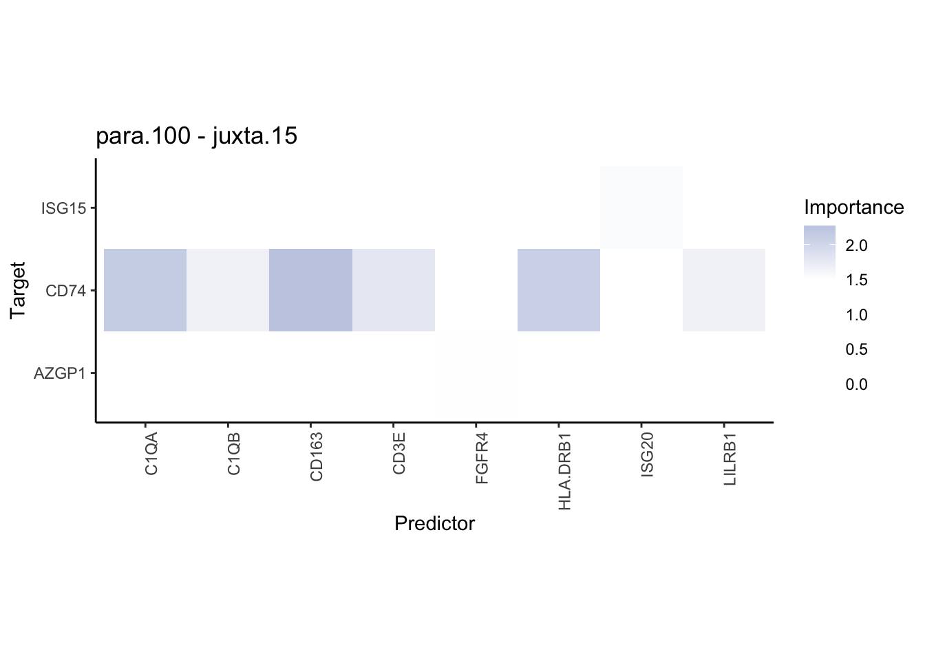
  plot_contrast_heatmap("juxta.15", "para.100", cutoff = 1.5, trim = 2)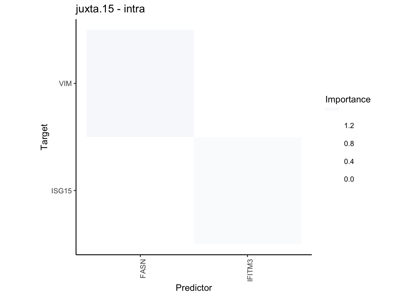
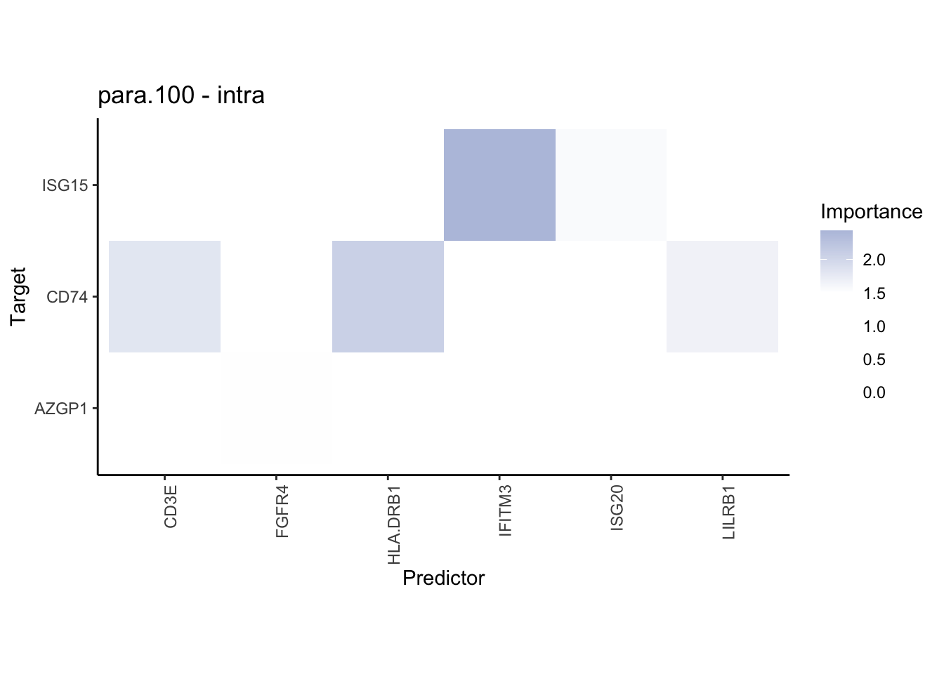
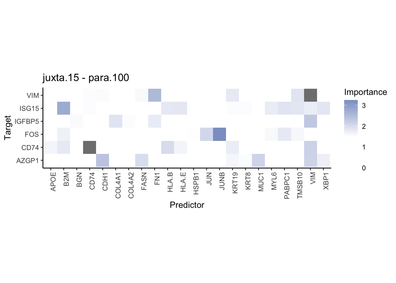
| Version | Author | Date |
|---|---|---|
| ec6405d | Jovan Tanevski | 2021-10-29 |
Plot interaction communities
misty.results.merfish %>%
  plot_interaction_communities("intra", cutoff = 6) %>%
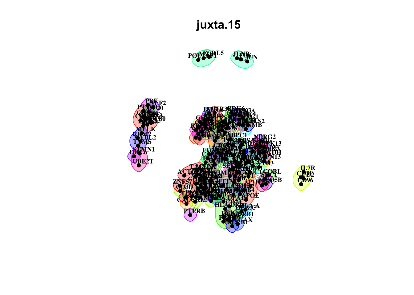
  plot_interaction_communities("juxta.15", cutoff = 2) %>%
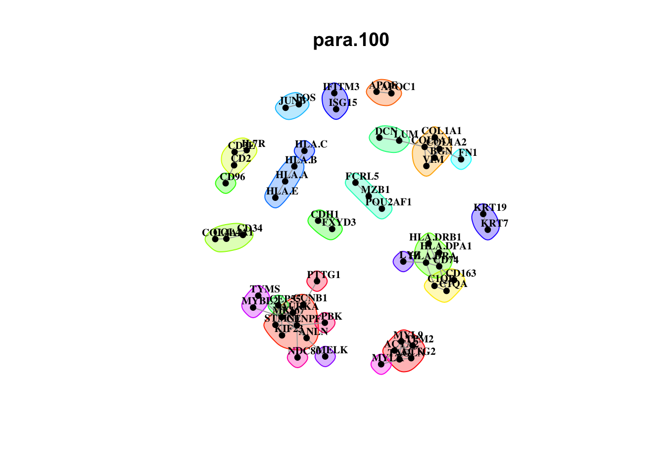
  plot_interaction_communities("para.100", cutoff = 2)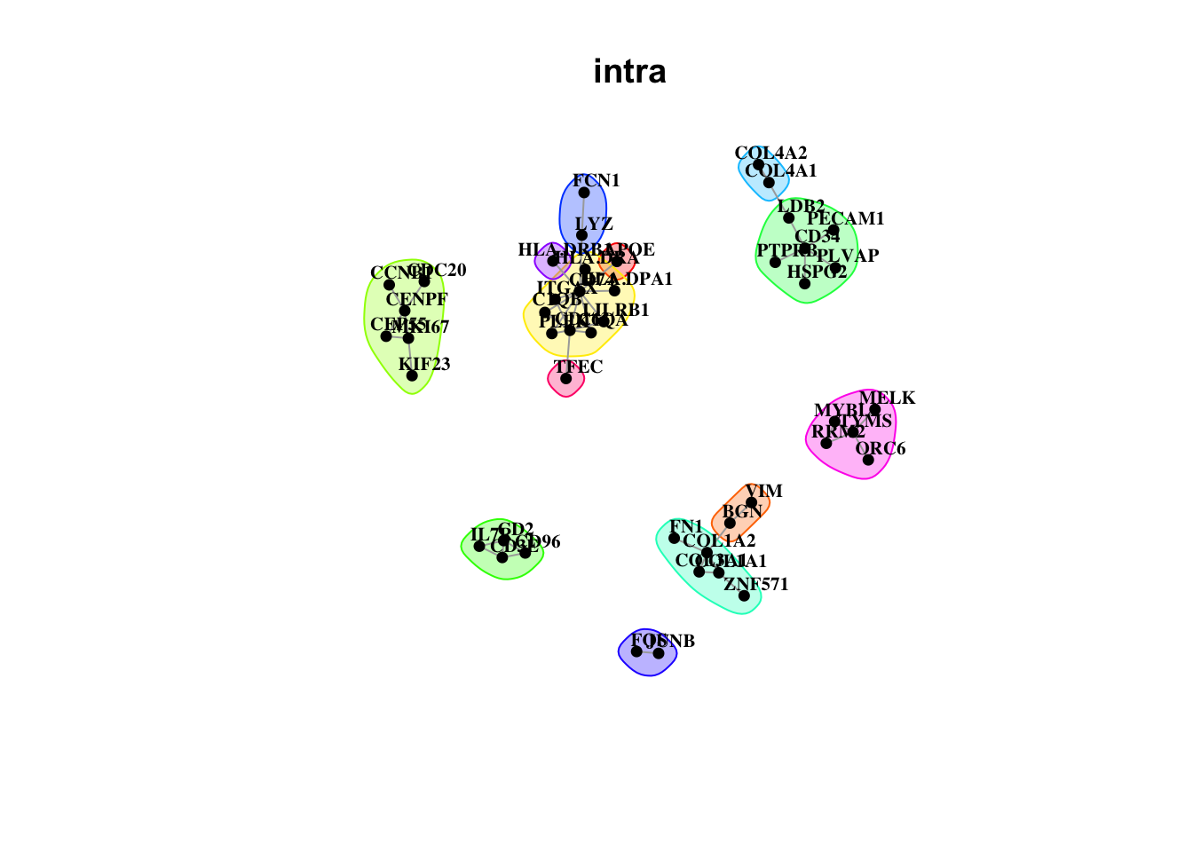
Signatures and clustering
We observe better clustering based on biopsy site than receptor status
signature.per.merfish <- misty.results.merfish %>%
  extract_signature("performance", trim = 2) %>%
  mutate(sample = str_extract(sample, "HTAPP(-[:alnum:]+){3}"))

signature.per.pca <- signature.per.merfish %>%
  select(-sample) %>%
  prcomp()

signature.per.pca.ann <- left_join(bind_cols(
  signature.per.merfish %>% select(sample),
  as.data.frame(signature.per.pca$x)
),
sample.meta,
by = c("sample" = "name")
)

ggplot(signature.per.pca.ann, aes(x = PC1, y = PC2)) +
  geom_point(aes(color = site_biopsy)) +
  theme_classic()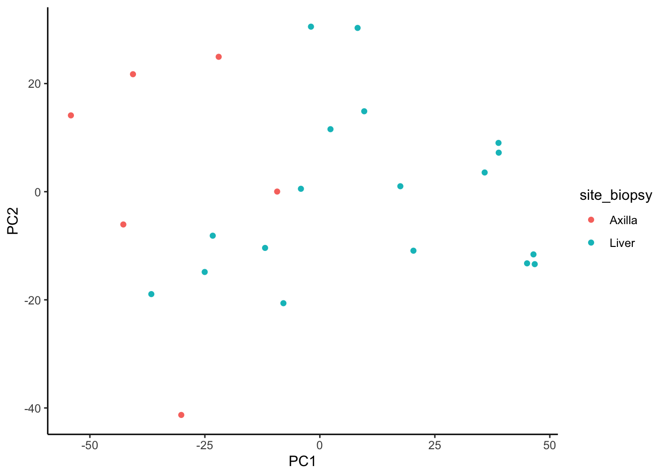
ggplot(signature.per.pca.ann, aes(x = PC1, y = PC2)) +
  geom_point(aes(color = receptors_biopsy)) +
  theme_classic()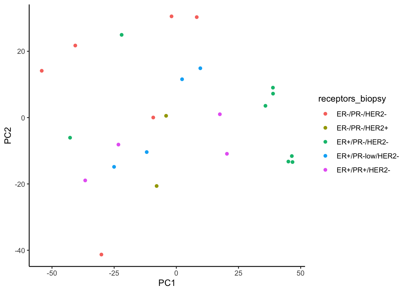
fviz_pca_var(signature.per.pca, col.var = "cos2", gradient.cols = c("#666666", "#377EB8", "#E41A1C"), repel = TRUE) + theme_classic()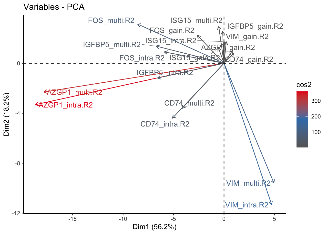
| Version | Author | Date |
|---|---|---|
| ec6405d | Jovan Tanevski | 2021-10-29 |
Compare samples from liver biopsies to all other
merfish.liver <- str_subset(outputs, "merfish") %>%
  str_subset(sample.meta %>%
               filter(site_biopsy == "Liver") %>%
               pull(name) %>%
               str_extract("\\d+$") %>%
               paste0(.,collapse = "|"))

merfish.other <- str_subset(outputs, "merfish") %>%
  str_subset(sample.meta %>%
               filter(site_biopsy != "Liver") %>%
               pull(name) %>%
               str_extract("\\d+$") %>%
               paste0(.,collapse = "|"))

results.merfish.liver <- collect_results(merfish.liver)
Collecting improvements
Collecting contributions
Collecting importances
Aggregatingresults.merfish.other <- collect_results(merfish.other)
Collecting improvements
Collecting contributions
Collecting importances
Aggregatingresults.merfish.liver %>% plot_improvement_stats(trim = 2)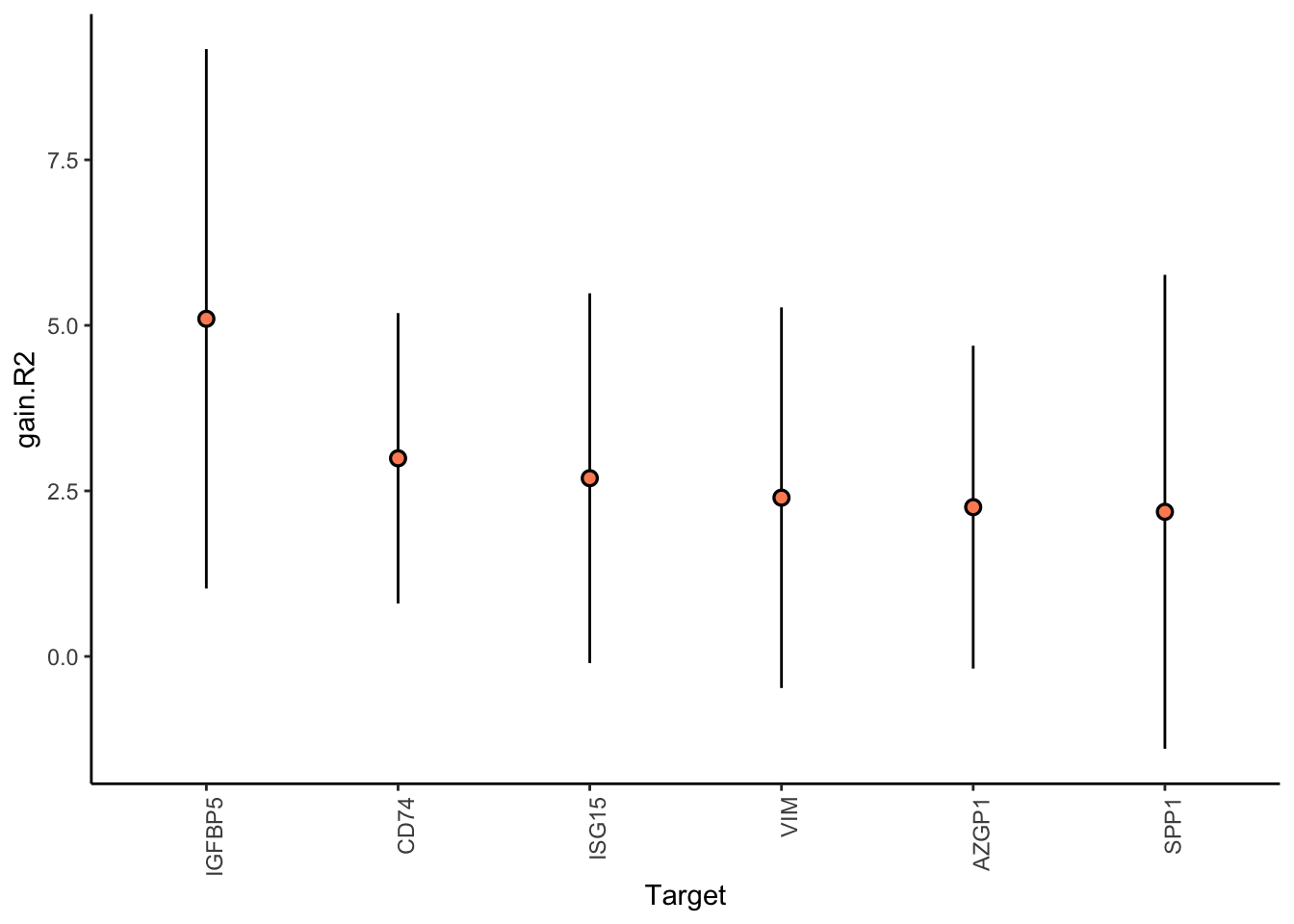
results.merfish.other %>% plot_improvement_stats(trim = 2)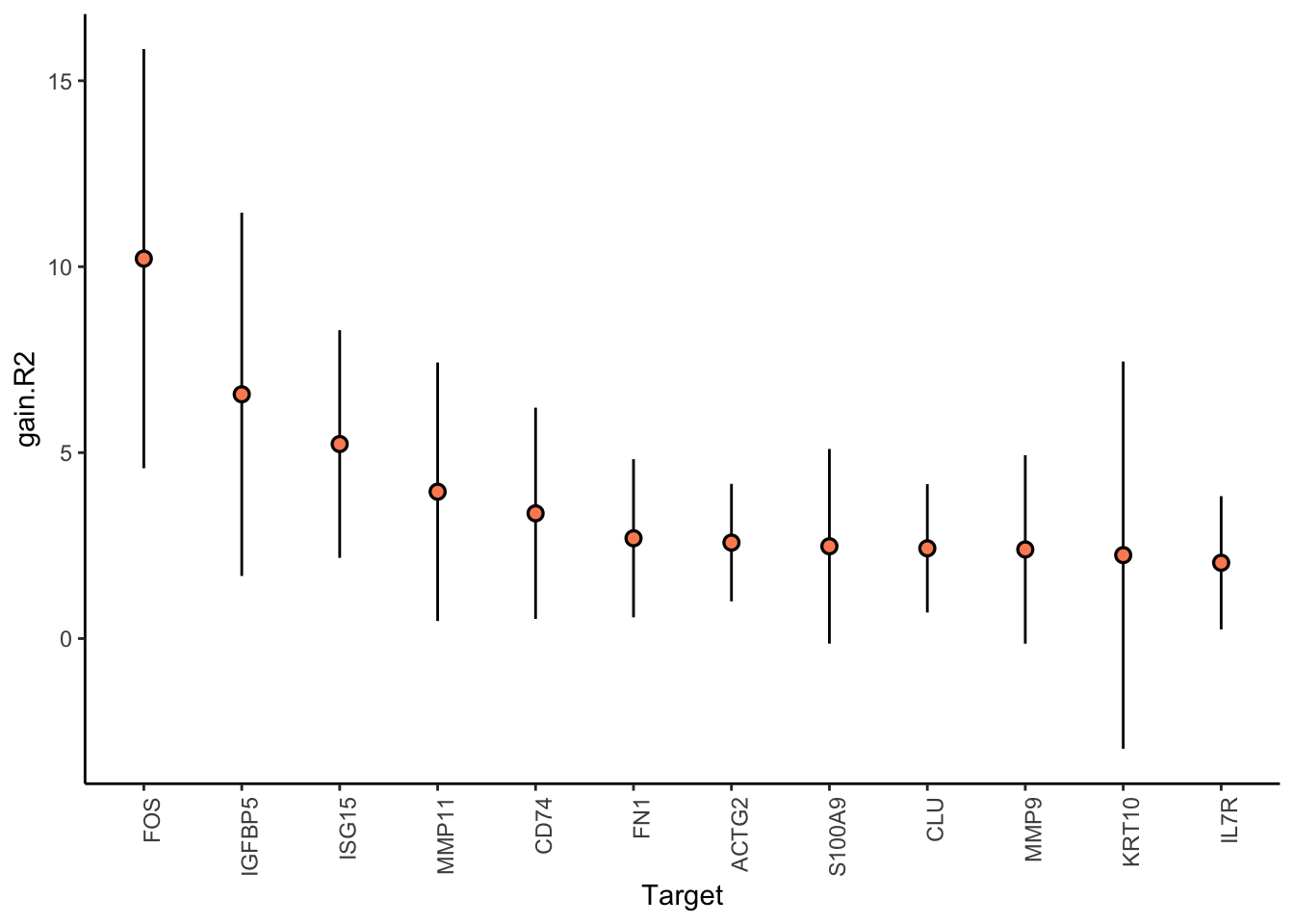
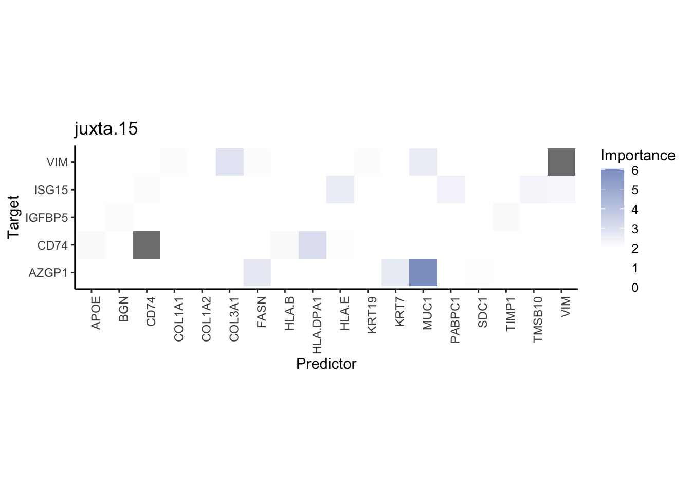
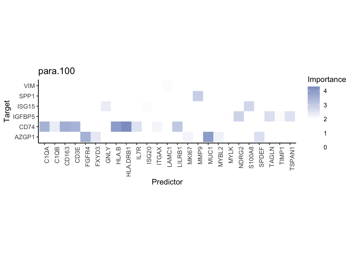
Liver specific interactions
plot_contrast_results(results.merfish.liver, results.merfish.other,
                      cutoff.from = 2, cutoff.to = 2, trim = 2)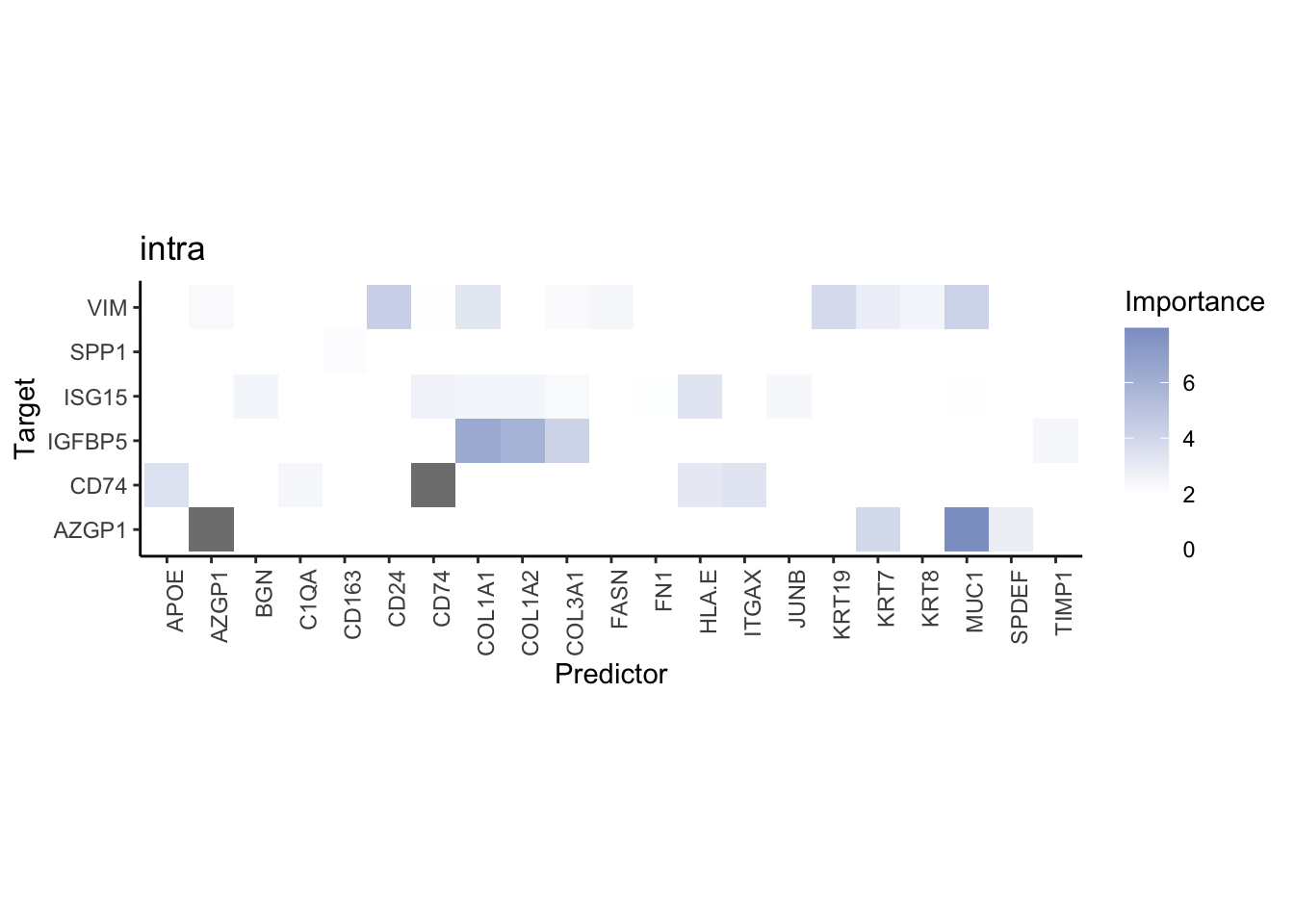
Merge CODEX and MERFISH results
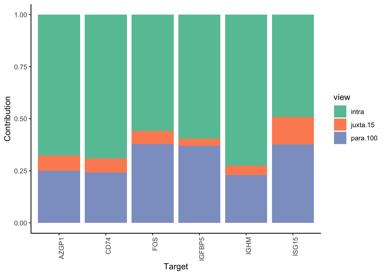
Filter only genes with mean gain in variance explained of 1 or more to plot the gain and view contributions
misty.results.merged <- collect_results(str_subset(outputs, "(codex|merfish)"))
Collecting improvements
Collecting contributions
Collecting importances
Aggregatingmisty.results.merged %>%
plot_improvement_stats(trim = 2) %>%
plot_view_contributions(trim = 2)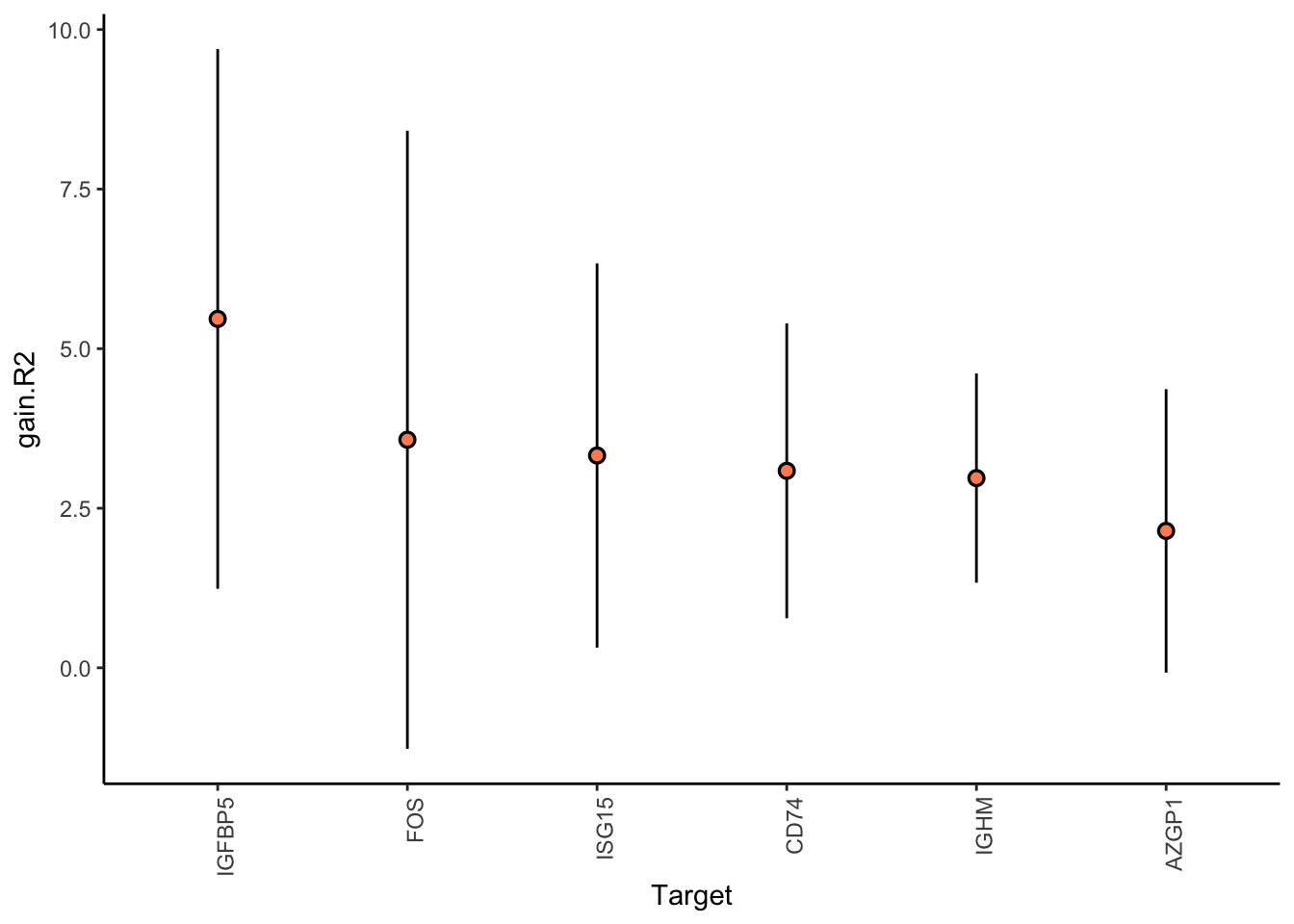
| Version | Author | Date |
|---|---|---|
| ec6405d | Jovan Tanevski | 2021-10-29 |
Plot interaction heatmaps
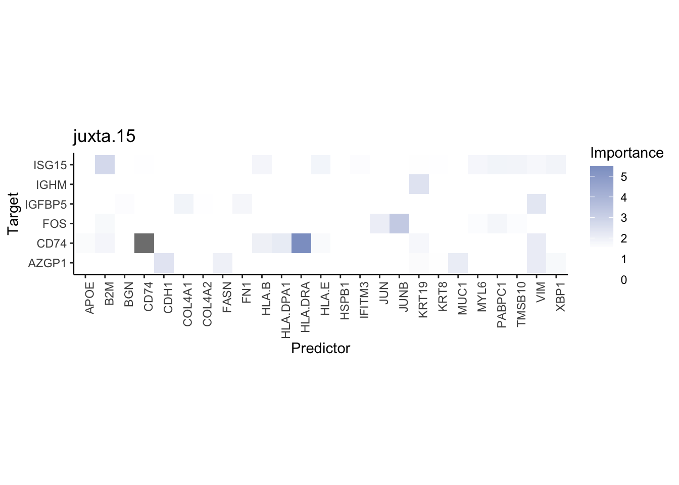
misty.results.merged %>%
  plot_interaction_heatmap("intra", cutoff = 8, clean = TRUE) %>%
  plot_interaction_heatmap("juxta.15", cutoff = 1.5, clean = TRUE, trim = 2) %>%
  plot_interaction_heatmap("para.100", cutoff = 1.5, clean = TRUE, trim = 2) %>%
  plot_contrast_heatmap("intra", "juxta.15", cutoff = 1.5, trim = 2) %>%
  plot_contrast_heatmap("intra", "para.100", cutoff = 1.5, trim = 2)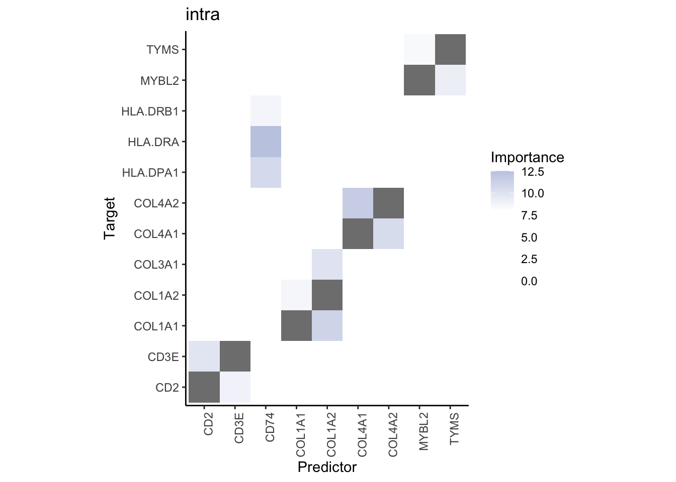
| Version | Author | Date |
|---|---|---|
| ec6405d | Jovan Tanevski | 2021-10-29 |
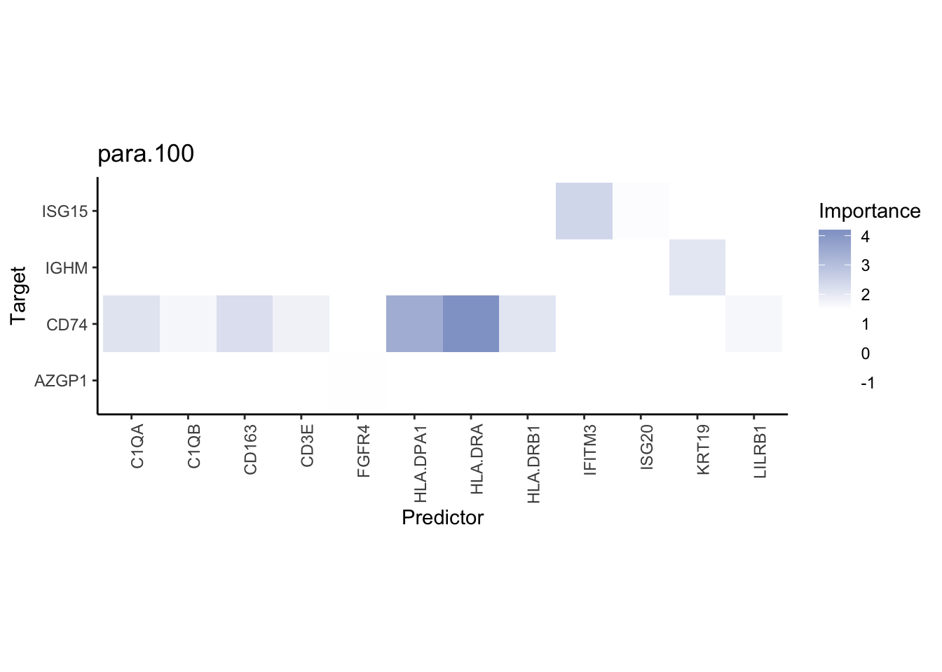
| Version | Author | Date |
|---|---|---|
| ec6405d | Jovan Tanevski | 2021-10-29 |
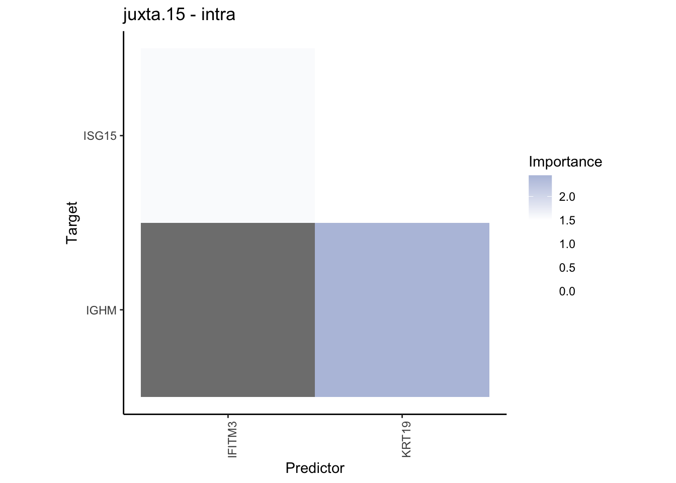
| Version | Author | Date |
|---|---|---|
| ec6405d | Jovan Tanevski | 2021-10-29 |
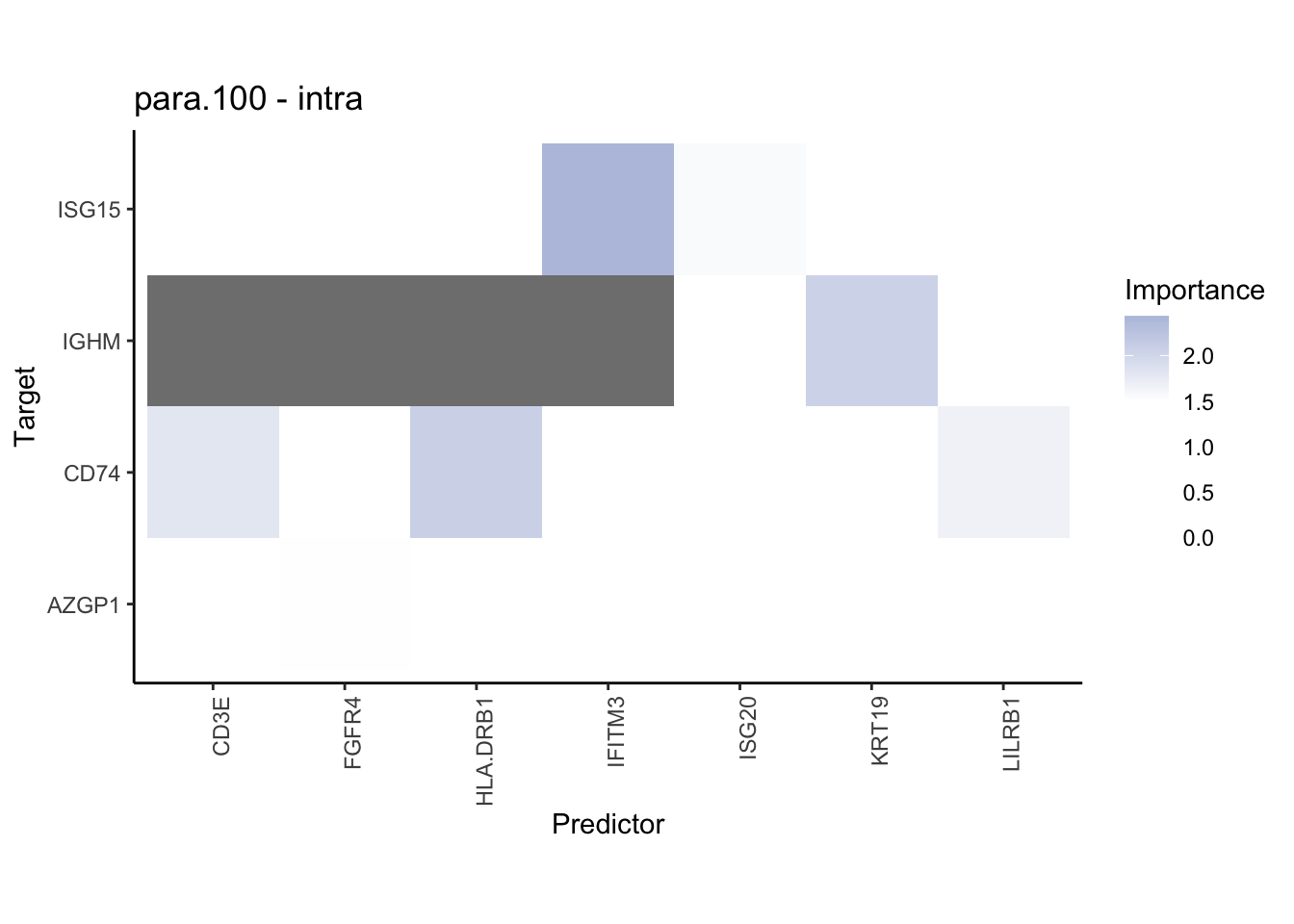
| Version | Author | Date |
|---|---|---|
| ec6405d | Jovan Tanevski | 2021-10-29 |
Signatures
There are no common targets with improvements above 1% between the two technologies, therefore we extract the signature using all markers, although we expect to have a technology based batch effect.
sig.perf <- extract_signature(misty.results.merged, "performance")
sig.perf.pca <- sig.perf %>%
  select(-sample) %>%
  prcomp()

sig.perf.join <- sig.perf %>%
  mutate(
    tech = str_extract(sample, "(merfish_processed|merfish_bin|codex)"),
    sample = str_extract(sample, "HTAPP-[0-9]{3}-SMP-[0-9]{3,4}")
  ) %>%
  select(tech, sample) %>%
  bind_cols(as.data.frame(sig.perf.pca$x)) %>%
  left_join(sample.meta, by = c("sample" = "name"))

ggplot(sig.perf.join, aes(x = PC1, y = PC2)) +
  geom_point(aes(color = tech)) +
  theme_classic()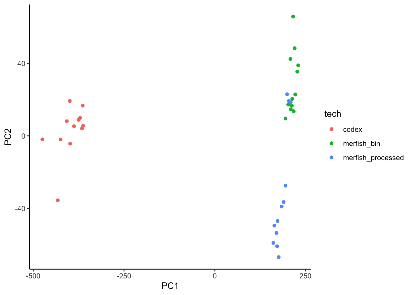
ggplot(sig.perf.join, aes(x = PC1, y = PC2)) +
  geom_point(aes(color = site_biopsy)) +
  theme_classic()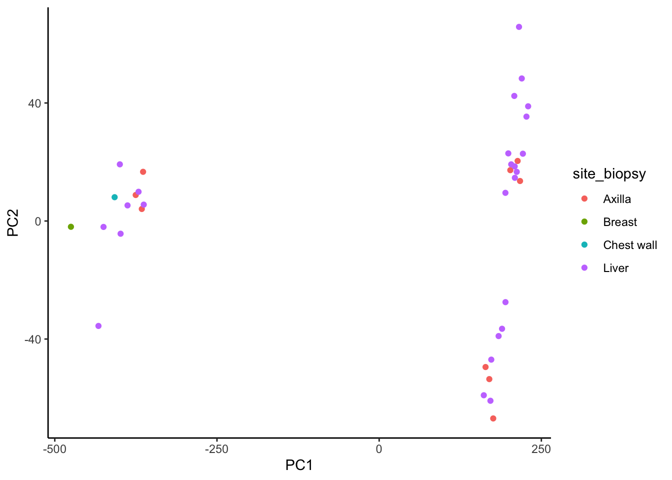
SlideSeq
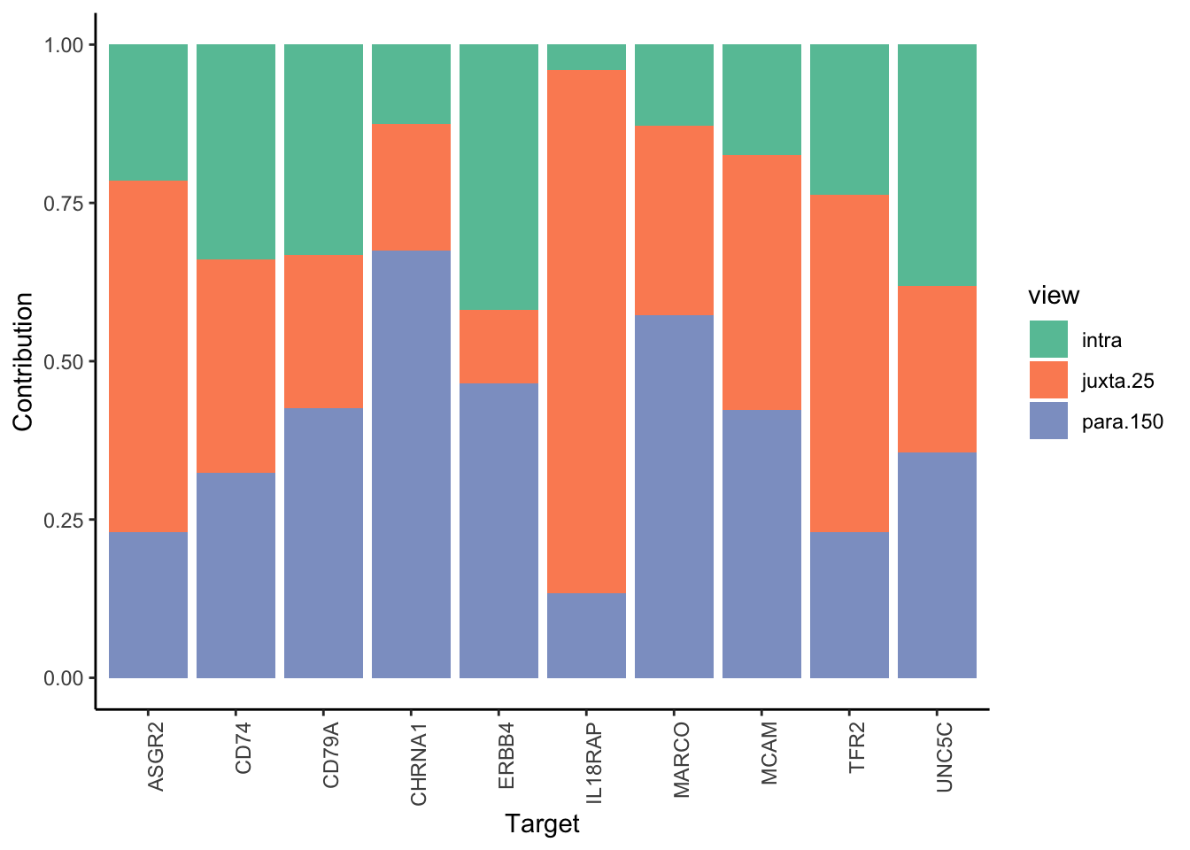
Filter only ligands then pathways with mean gain in variance explained of 1 or more to plot the gain and view contributions
misty.results.ligrcp %>%
  plot_improvement_stats(trim = 0.5) %>%
  plot_view_contributions(trim = 0.5)
Warning: Removed 1 rows containing missing values (geom_segment).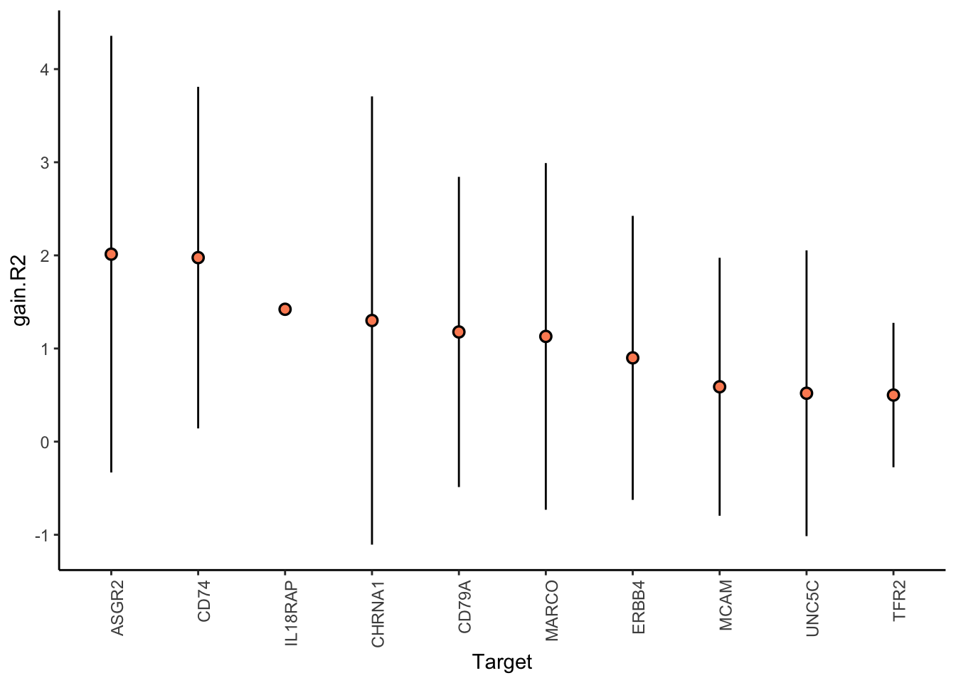
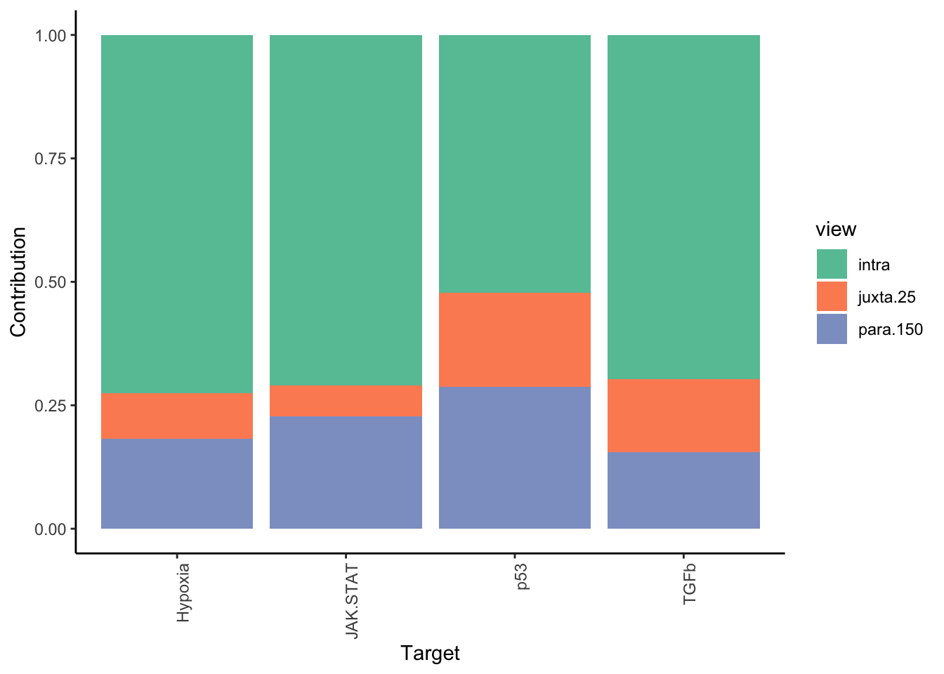
misty.results.ligpath %>%
  plot_improvement_stats(trim = 1) %>%
  plot_view_contributions(trim = 1)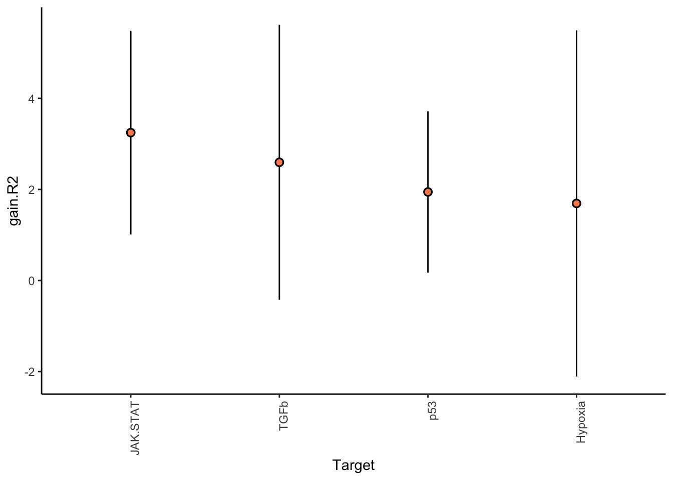
Plot interaction heatmaps
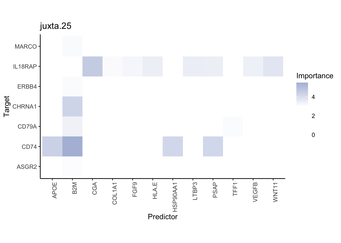
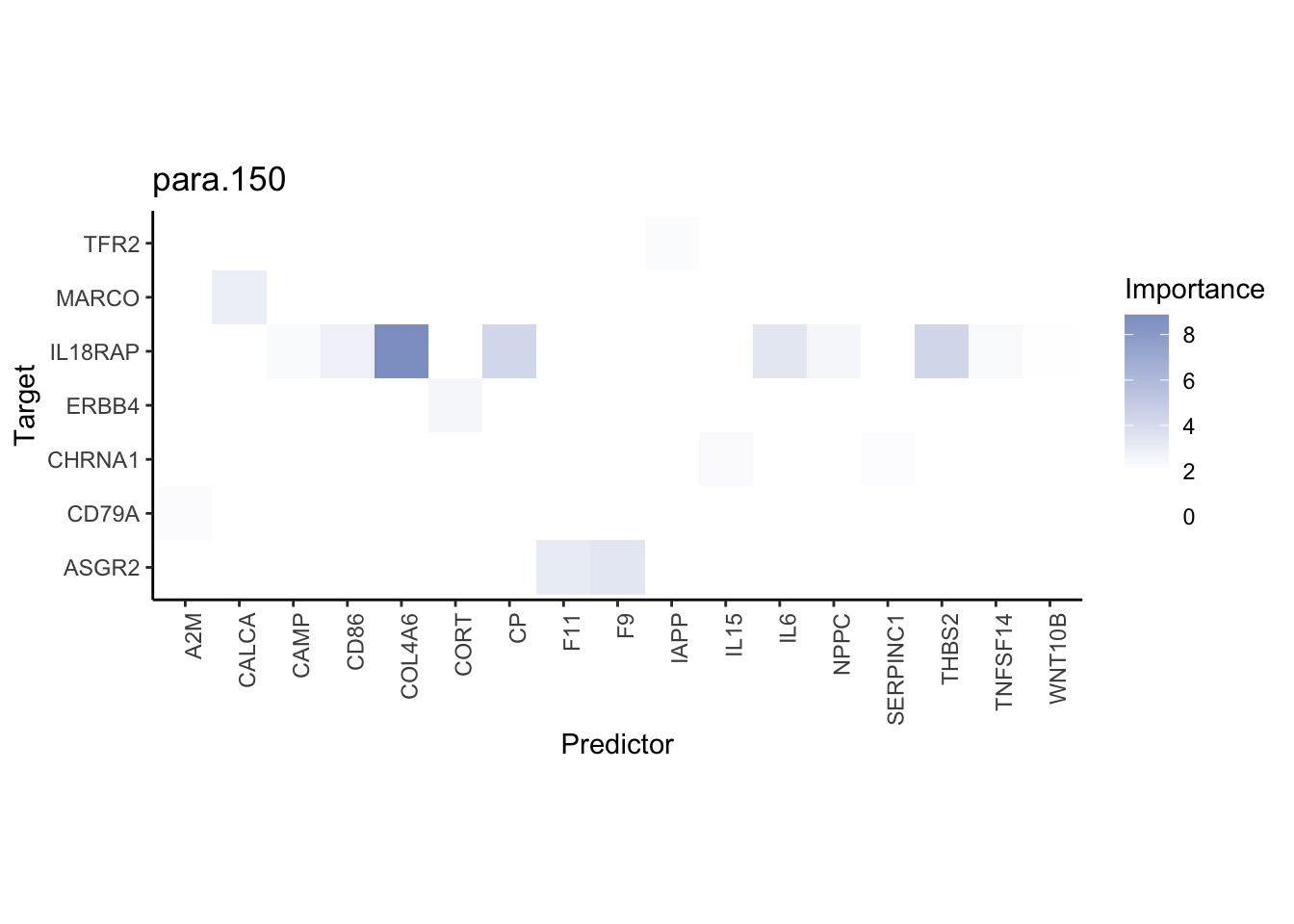
misty.results.ligrcp %>%
  plot_interaction_heatmap("intra", cutoff = 5, clean = TRUE) %>%
  plot_interaction_heatmap("juxta.25", cutoff = 3, clean = TRUE, trim = 0.5) %>%
  plot_interaction_heatmap("para.150", cutoff = 2, clean = TRUE, trim = 0.5)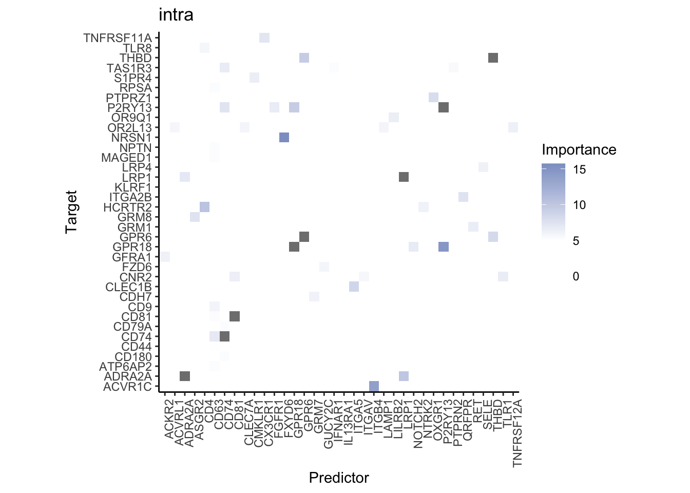
| Version | Author | Date |
|---|---|---|
| ec6405d | Jovan Tanevski | 2021-10-29 |
| Version | Author | Date |
|---|---|---|
| ec6405d | Jovan Tanevski | 2021-10-29 |
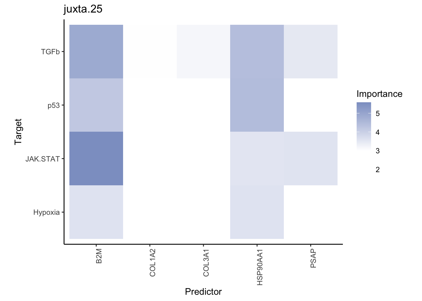
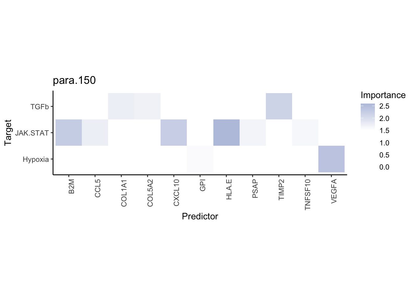
misty.results.ligpath %>%
  plot_interaction_heatmap("intra", cutoff = 1.5, clean = TRUE) %>%
  plot_interaction_heatmap("juxta.25", cutoff = 3, clean = TRUE, trim = 1) %>%
  plot_interaction_heatmap("para.150", cutoff = 1.5, clean = TRUE, trim = 1)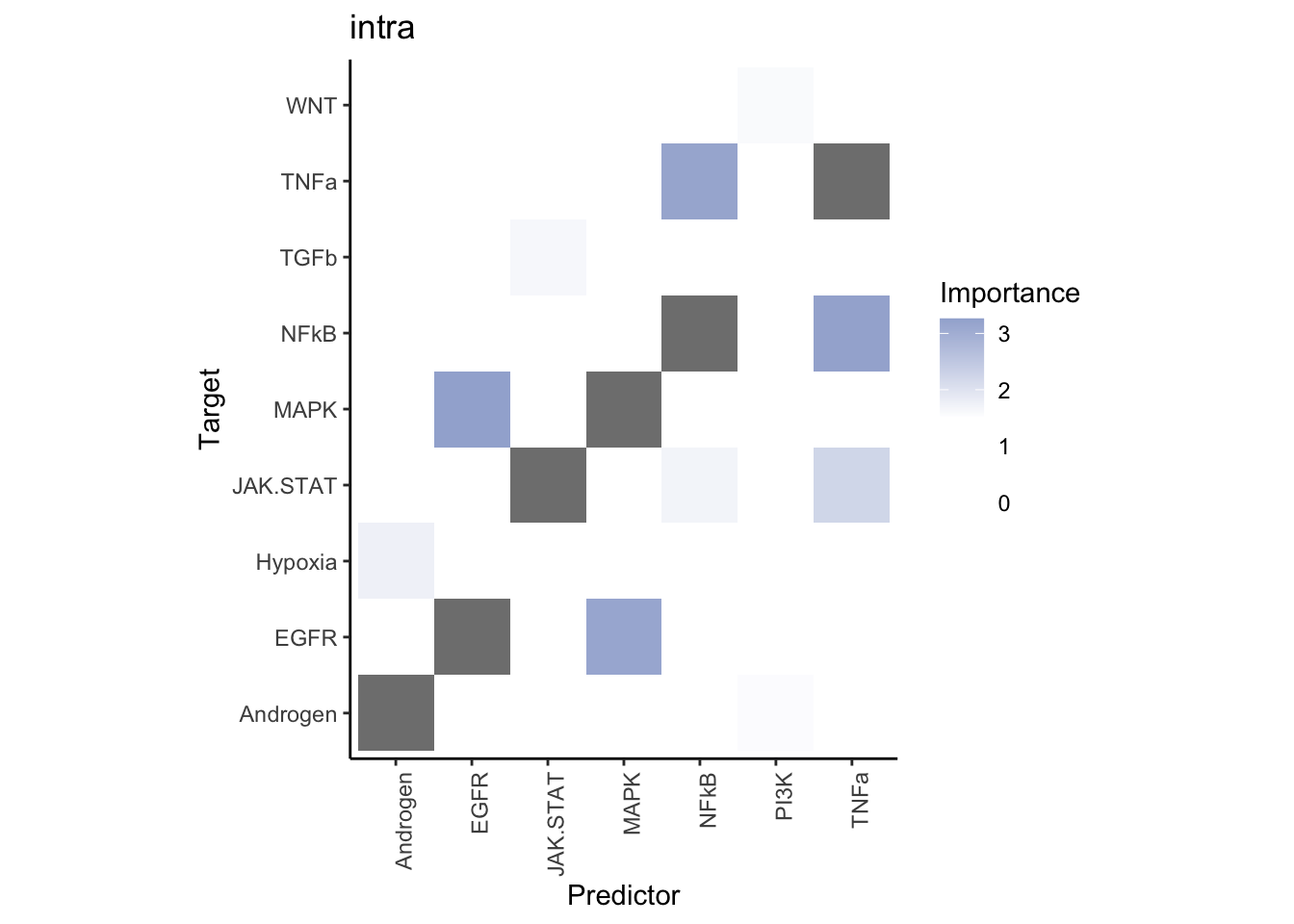
Plot intrinsic pathway communities
misty.results.ligpath %>% plot_interaction_communities("intra", cutoff = 1.5)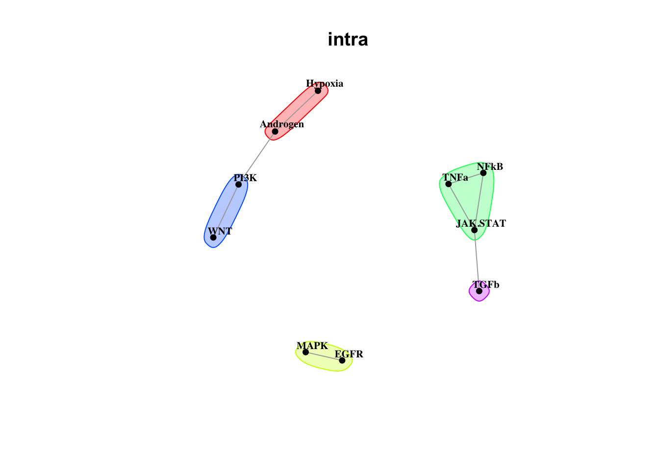
| Version | Author | Date |
|---|---|---|
| ec6405d | Jovan Tanevski | 2021-10-29 |
Cell-type based analysis
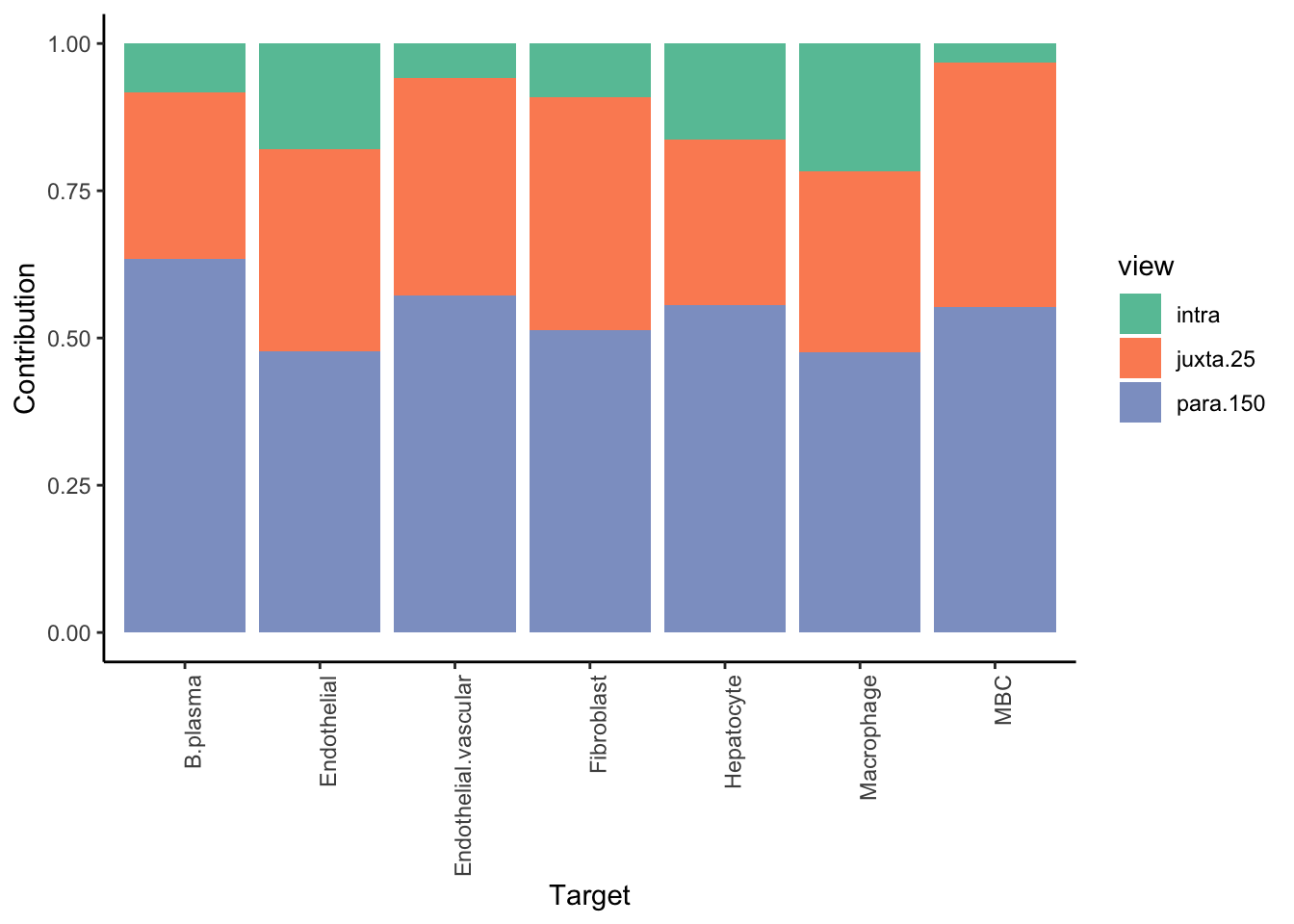
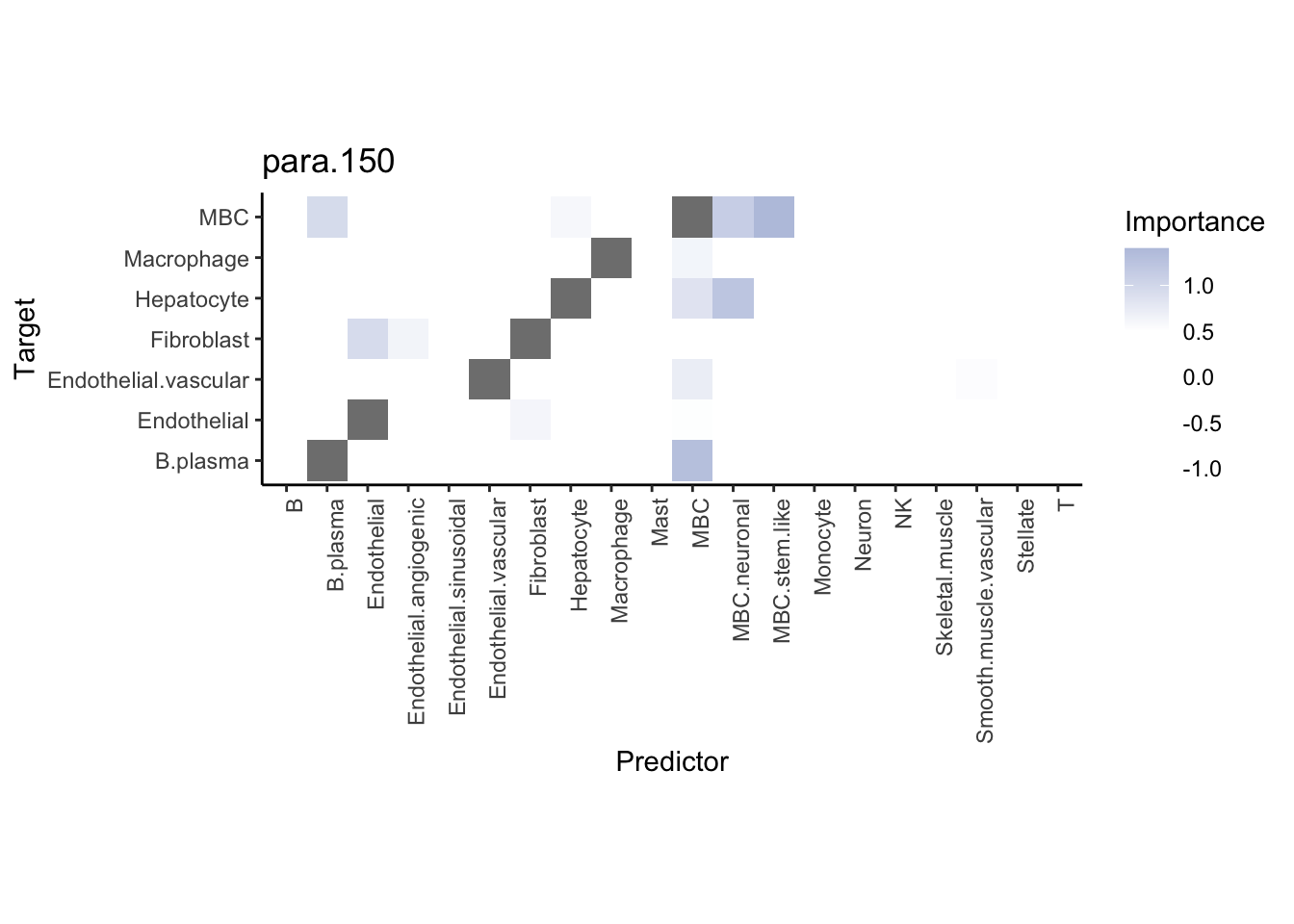
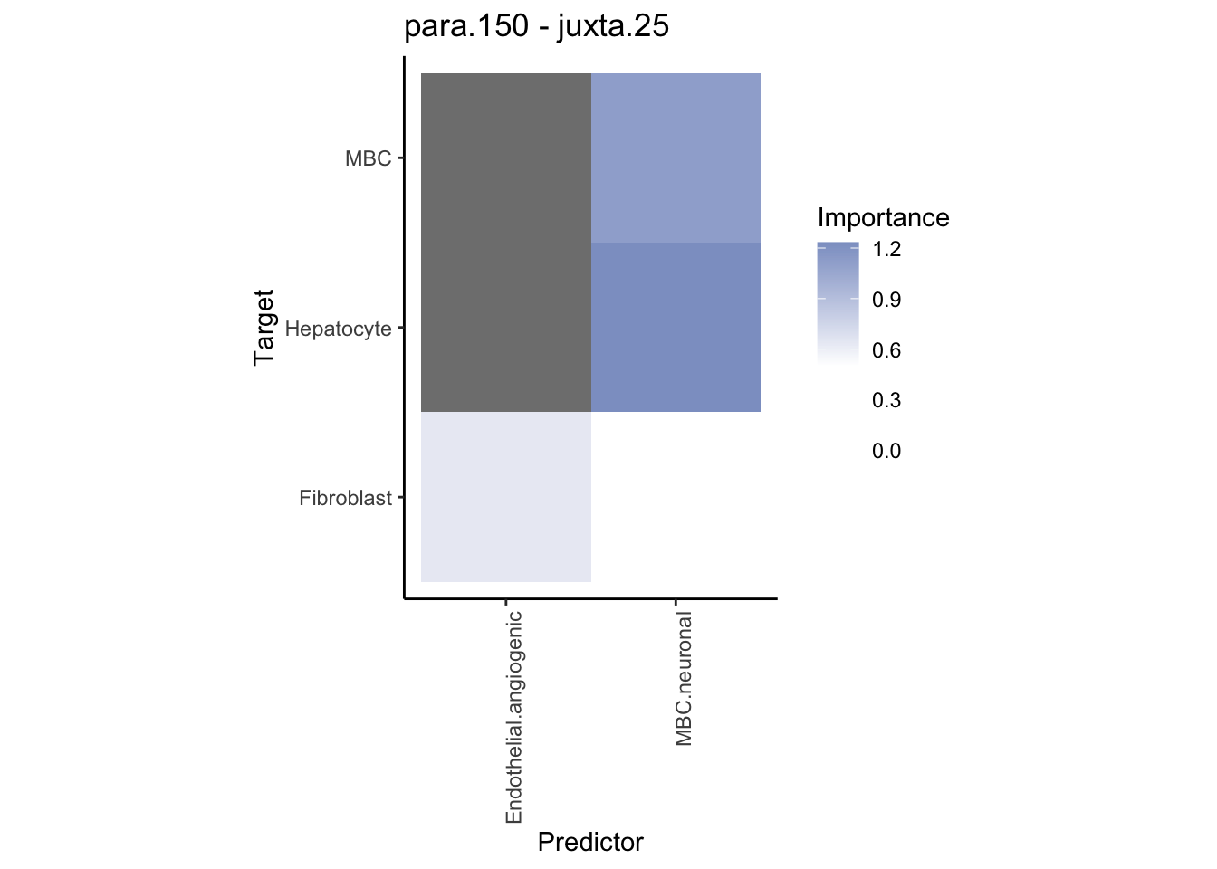
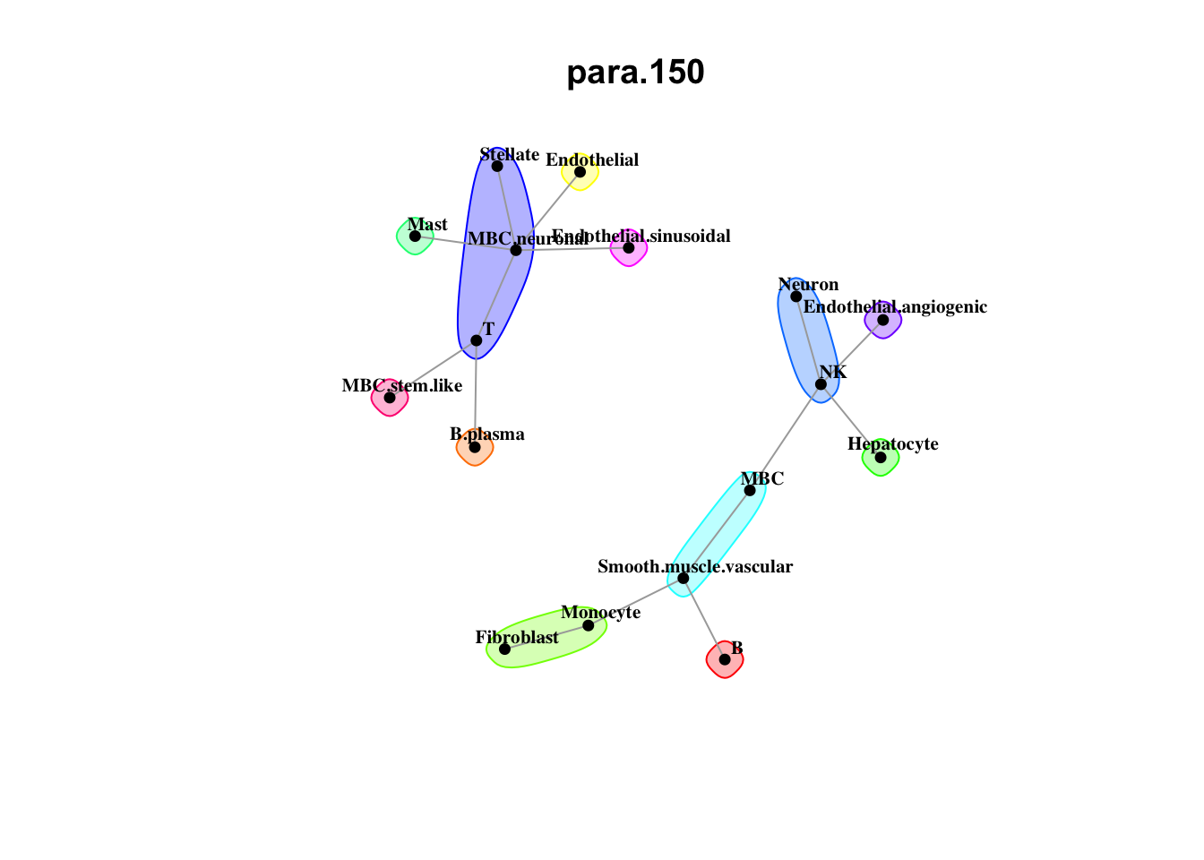
We are interested in predicting the probability of a cell being of a cell-type of interest, by looking at the distribution of cell types in the neighborhood of 100 cells.
More conservative trimming of above 10% variance explained since the intraview is bypassed. The contribution of the intraview can be interpreted as the amount of variance captured only by the mean of the probability estimate for that cell-type. For a good result it is expected to be close to zero.
misty.results.ctype <- collect_results(str_subset(outputs, "ctype"))
Collecting improvements
Collecting contributions
Collecting importances
Aggregatingmisty.results.ctype %>%
plot_improvement_stats(trim = 10) %>%
plot_view_contributions(trim = 10)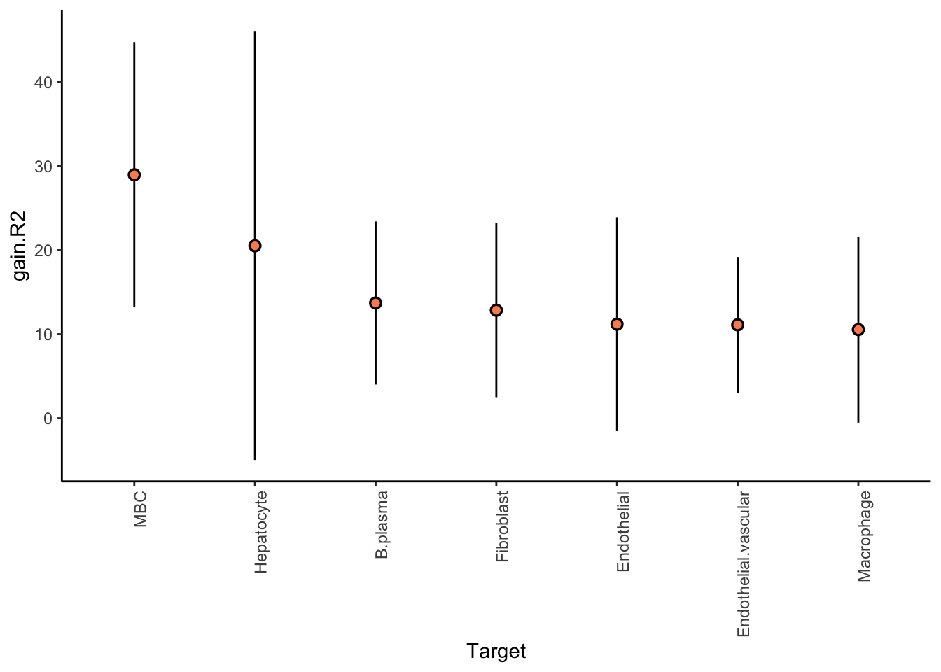
Plot neighborhood interactions
misty.results.ctype %>%
  plot_interaction_heatmap("juxta.25", trim = 10, cutoff = 0.5) %>%
  plot_interaction_heatmap("para.150", trim = 10, cutoff = 0.5)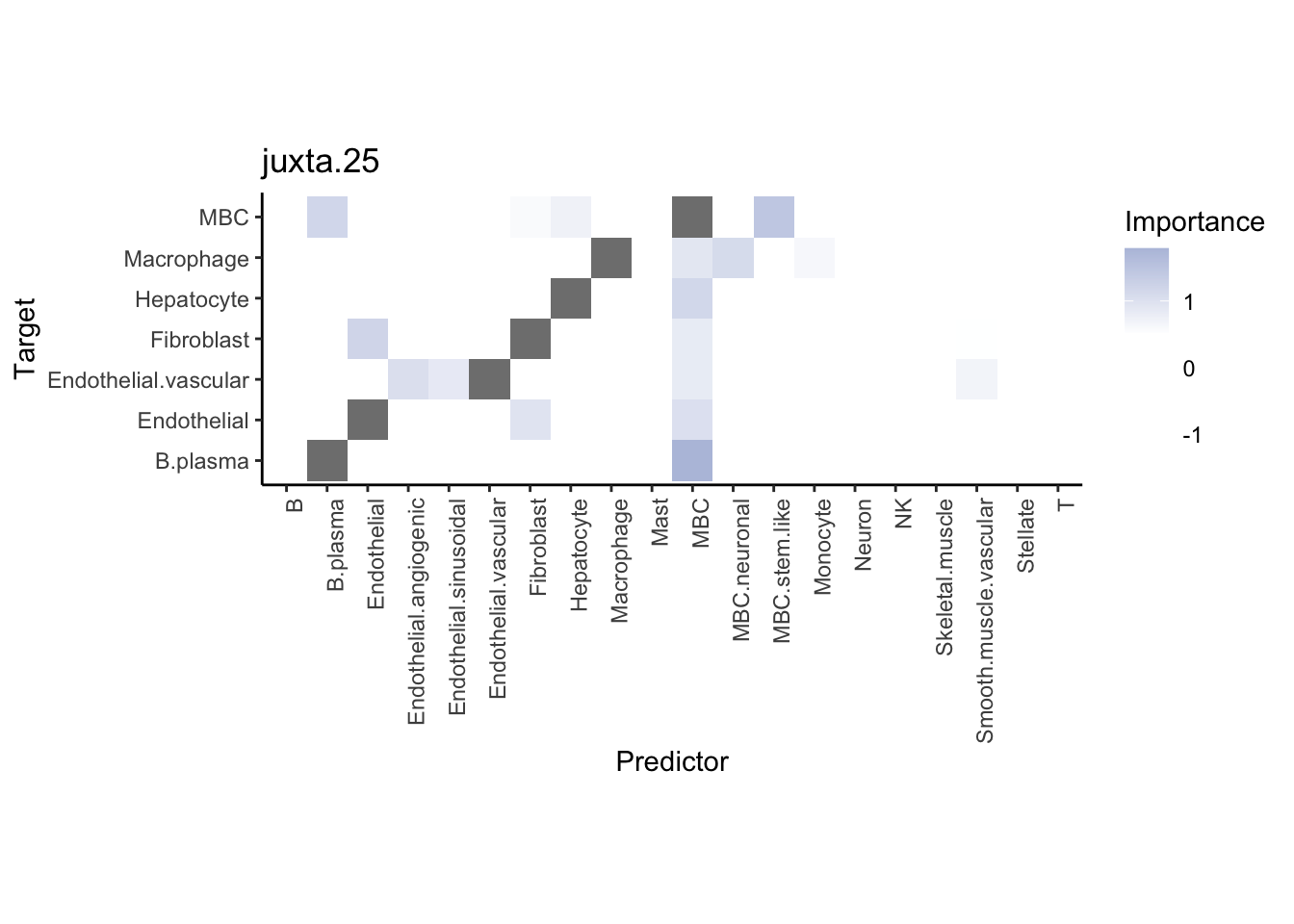
Plot contrasts
misty.results.ctype %>%
  plot_contrast_heatmap("para.150", "juxta.25", trim = 10, cutoff = 0.5) %>%
  plot_contrast_heatmap("juxta.25", "para.150", trim = 10, cutoff = 0.5)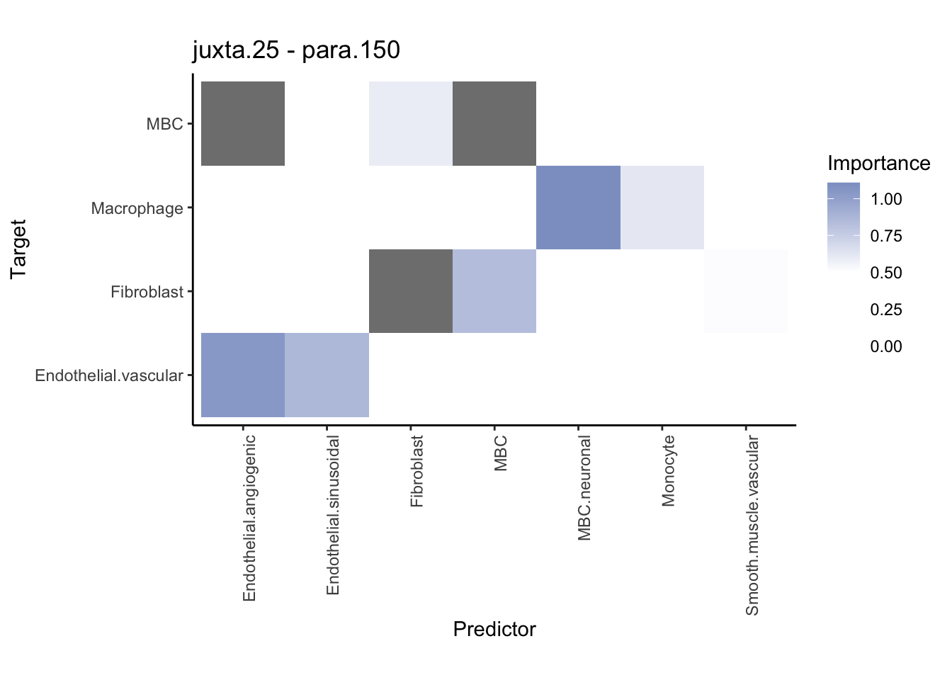
Plot communities
misty.results.ctype %>%
  plot_interaction_communities("juxta.25", cutoff = 1) %>%
  plot_interaction_communities("para.150", cutoff = 1)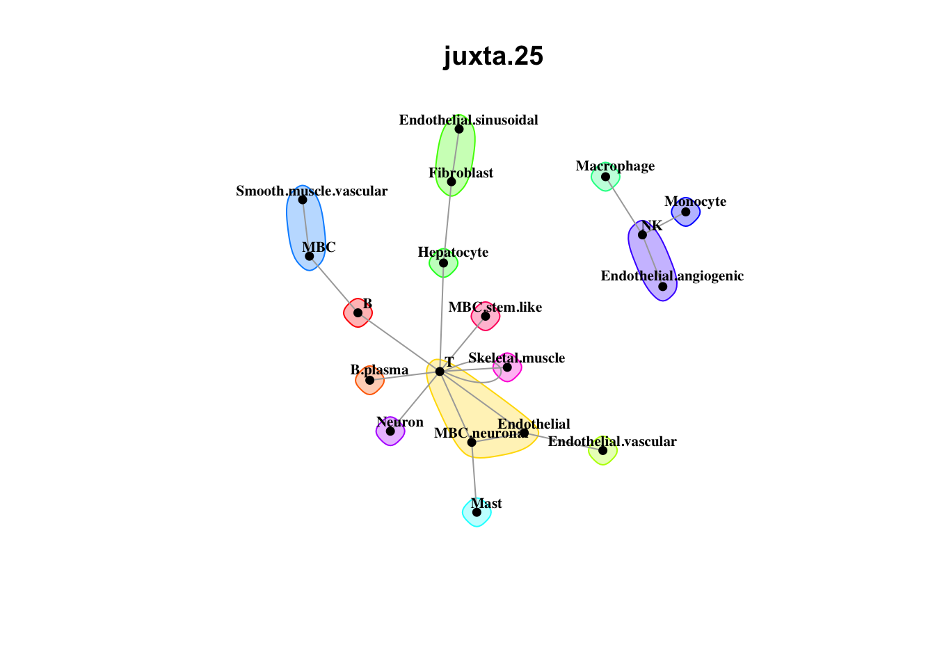
sessionInfo()R version 4.1.2 (2021-11-01)
Platform: x86_64-apple-darwin17.0 (64-bit)
Running under: macOS Big Sur 10.16
Matrix products: default
BLAS: /Library/Frameworks/R.framework/Versions/4.1/Resources/lib/libRblas.0.dylib
LAPACK: /Library/Frameworks/R.framework/Versions/4.1/Resources/lib/libRlapack.dylib
locale:
[1] en_US.UTF-8/en_US.UTF-8/en_US.UTF-8/C/en_US.UTF-8/en_US.UTF-8
attached base packages:
[1] stats graphics grDevices utils datasets methods base
other attached packages:
[1] factoextra_1.0.7 future_1.23.0 ggplot2_3.3.5 mistyR_1.3.5
[5] readr_2.1.1 dplyr_1.0.7 stringr_1.4.0 workflowr_1.7.0
loaded via a namespace (and not attached):
[1] ggrepel_0.9.1 Rcpp_1.0.8 tidyr_1.1.4 listenv_0.8.0
[5] getPass_0.2-2 ps_1.6.0 assertthat_0.2.1 rprojroot_2.0.2
[9] digest_0.6.29 utf8_1.2.2 parallelly_1.30.0 R6_2.5.1
[13] backports_1.4.1 evaluate_0.14 highr_0.9 httr_1.4.2
[17] pillar_1.6.4 rlang_0.4.12 rstudioapi_0.13 car_3.0-12
[21] furrr_0.2.3 whisker_0.4 callr_3.7.0 jquerylib_0.1.4
[25] R.utils_2.11.0 R.oo_1.24.0 rmarkdown_2.11 labeling_0.4.2
[29] igraph_1.2.11 munsell_0.5.0 broom_0.7.11 compiler_4.1.2
[33] httpuv_1.6.5 xfun_0.29 pkgconfig_2.0.3 globals_0.14.0
[37] htmltools_0.5.2 tidyselect_1.1.1 tibble_3.1.6 codetools_0.2-18
[41] fansi_1.0.2 ggpubr_0.4.0 crayon_1.4.2 tzdb_0.2.0
[45] withr_2.4.3 later_1.3.0 R.methodsS3_1.8.1 grid_4.1.2
[49] jsonlite_1.7.3 gtable_0.3.0 lifecycle_1.0.1 DBI_1.1.2
[53] git2r_0.29.0 magrittr_2.0.1 scales_1.1.1 carData_3.0-5
[57] stringi_1.7.6 ggsignif_0.6.3 farver_2.1.0 fs_1.5.2
[61] promises_1.2.0.1 bslib_0.3.1 ellipsis_0.3.2 generics_0.1.1
[65] vctrs_0.3.8 RColorBrewer_1.1-2 tools_4.1.2 glue_1.6.1
[69] purrr_0.3.4 hms_1.1.1 abind_1.4-5 processx_3.5.2
[73] parallel_4.1.2 fastmap_1.1.0 yaml_2.2.1 colorspace_2.0-2
[77] rstatix_0.7.0 knitr_1.37 sass_0.4.0