Running CellNOpt requires the igraph package to be installed, while in addition for running the CNORode package the MEIGO optimization toolbox needs also to be installed first.
CellNOpt method derives a logic-based model from a prior knowledge network (PKN) and trains it against perturbation measurements. The PKN is typically inferred from information from literature or expert knowledge and then tests this prior knowledge if it is compatible with the measurements in a specific perturbation context. All CNO formalisms, typically take two kind of inputs: i)A SIF (Simple Interaction File) text format which containing the PKN with the signed directed interactions happening between sites and which can be manipulated in Cytoscape and ii)A MIDAS (Minimum Information for Data Analysis in System Biology) containing data which are representing measurements of sites upon various stimuli and inhibitory perturbations.
To prepare the prior knowledge network for training, we first apply two pre-processing steps: i)In compression we reduce and simplify the network by removing species that are neither measured nor perturbed without impairing tha logical consistency of the network. ii)In expansion all the logical operations from each interactions are added.
Training involves the identification of the sub-models of the processed $PKN$ which better explains and fits the data by minimizing the mean squared deviation $ \theta_f $ between model prediction $ B^{M} $ and the actual measurements $ B^{E} $ for the $ m $ readouts, $ n $ time-points and $ s $ experimental conditions weighted by the total number of data points $ n_{g} $.
\[\theta_f(P) = \frac{1}{n_{g}} \sum_{k=1}^{s} \sum_{l=1}^{m} \sum_{t=1}^{n} (B_{k,l,t}^{M}-B_{k,l,t}^{E})^{2}\]$ P $ on this case, represent one of the solutions or the string of bits indicating whether an edge of the compressed network is included in the model or not.
We also add a size penalty $ \theta_s $ to the objective function as the sum of the number of inputs $ \nu_{e} $ of each edge $ e $ in $ P $ normalized by the total number of inputs across all edges (\(\nu _{e}^{s} = \sum_{e=1}^{r}\)) where $ r $ represents the length of $ P $.
\[\theta_s(P) = \frac{1}{\nu _{e}^{s}} \sum_{e=1}^{r}\nu _{e}P_{e}\]Networks inferred are written to a file and plotted, while information about the optimization during the training step are summarized in a central HTML report hyperlinked to the different plots.
The following is a Toy model Example as described in the documentation report of the CellNOptR package.
Initially we call our useful packages and then load the data and the prior knowledge.
library(CellNOptR)
library(igraph)

data("ToyModel", package="CellNOptR")
data("CNOlistToy", package="CellNOptR")
pknmodel = ToyModel
cnolist = CNOlist(CNOlistToy)

plotModel(model = pknmodel, CNOlist = cnolist)
The prior knowledge network will be plotted as follows:

As a second step, the model has to be pre-processed (commpressed and then expanded), before runnng the optimisation.
model = preprocessing(cnolist, pknmodel)

res = gaBinaryT1(cnolist, model, verbose=FALSE)
Results and the optimal sub-model then can then be plotted after calling the following functions:
cutAndPlot(cnolist, model, list(Res$bString))

plotModel(model, cnolist, res$bString)
Plot of the results:
Plot of the optimal model:
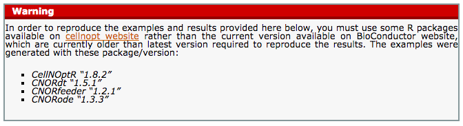
This tutorial is for advanced users. It combines the CellNOptR, CNORode and CNORfeeder packages. The goal of this tutorial is to provide the material to reproduce some results shown or discussed about in the SBMLqual paper, which is available in the arxiv.
The first part reproduces one of figure shown in the paper. This figure was reproduced by the different software used in the paper using the same SBMLqual model as input. Here, we show how one can use CellNOptR oftware to simulate the same dynamical states as the one shown in the paper.
The second part is more about CellNOptR software itself: we deal with the creation of some data sets (with CNORode), optimisation (with CNORdt) and usage of CNORfeeder to find missing links.
In CellNOptR, it is possible to load a SBMLqual file since version 1.7.8. Given the model, one can then decide to use different formalisms to simulate the dynamical states.
In this section, we provide a script called 2013/sbml/simulate.R that loads a SBMLqual and performs a simulation using another package called CNORdt. This package provide a discrete time formalism to simulate the dynamical states.
You can download the script from the link above and execute it as follows:
R script --no-save --no-restore < simulate.R
The SBMLqual file can be downloaded here: 2013/sbml/data/ModelV5.xml. The file is expected to be found in the directory: ./data. Otherwise you can change the script.
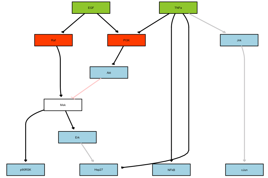
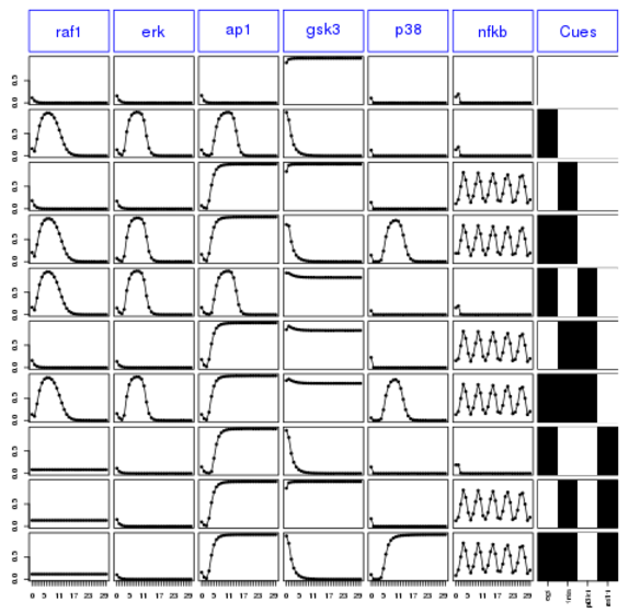
Each combination of stimuli lead to a different dynamical states. There are 4 combinations and therefore 4 pictures are generated. Here is one of them for which TNFa and EGF are stimulated:
In this section, we will do the following:
Using the same SBMLQual model as above, which we will call True model, we first generate the dynamical states using the ODE formalism (CNORode). The states are saved in MIDAS format.
Perform an optimisation (using CNORdt formalism) of the True model against the data for sanity check (the optimised model should be identical to the True model !!) and they fit almost perfect.
Then, we will create a Prior Knowledge Network (PKN) that is slightly different from the True model.
Using the PKN model and the data, we optimise the PKN model using a CNORdt formalism. We will see that there are discrepancies due to the differences between the True model and the PKN, in particular that there is a missing link in the PKN.
Finally, we will use CNORfeeder to infer the missing link based on the data. An optimisation will show that the CNORfeeder found the missing link.
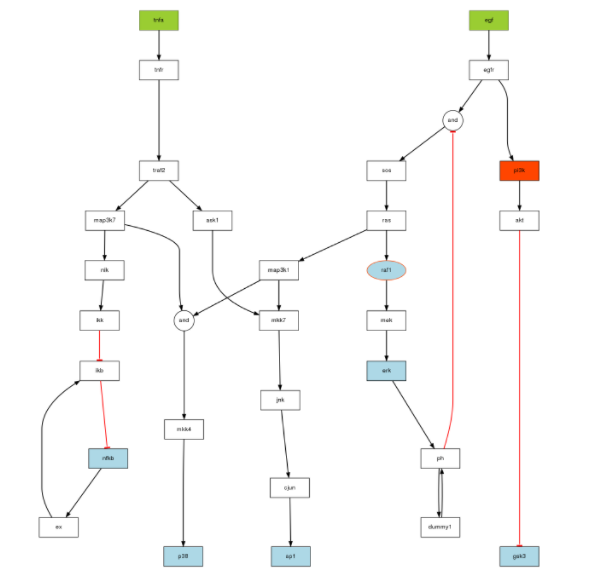
This example is based on the PKN and True model available [here] (http://iopscience.iop.org/1478-3975/9/4/045003)
Here is the code to generate the image corresponding to the True model:
library(CellNOptR)
model = readSBMLQual("ModelV5.xml")

library(CNORdt)
data(CNOlistPB, package="CNORdt")

plotModel(model, CNOlistPB)
To create the data using an ODE formalism, you will need a set of parameters available in 2013/sbml/data/paramsODE.RData.
library(CNORode) # for the simulation
library(CNORdt)  # for the data

data(CNOlistPB, package="CNORdt")

# Read the model with a dummy link on ph self loop
model = readSBMLQual("ModelV5.xml")

# load a variable called params that is required for the ODE run
load("paramsODE.RData")

timeSignals = seq(0,30,1)
CNOlistPB$timeSignals = seq(0,30,2)   # a trick to keep the original dt

# somehow stimuli set to exactly zero leads to NA so, replace them with
# tiny value but must set back to zero later on
CNOlistPB$valueStimuli[1,1] = 0.01
CNOlistPB$valueStimuli[1,2] = 0.01

sim_data = plotLBodeModelSim(CNOlistPB, model, ode_parameters=params,
    timeSignals=timeSignals, maxStepSize=0.035, show=F)
CNOlistPB$timeSignals = timeSignals

CNOlistPB$valueStimuli[1,1] = 0.
CNOlistPB$valueStimuli[1,2] = 0.

# finally converts the simdata to a cnolist to be saved in a file.
cnolist = simdata2cnolist(sim_data, CNOlistPB, model)

# keep only species of interest
species2select = c('raf1','erk', 'ap1', 'gsk3','p38', 'nfkb')
conditions2select = c(1,2,3,4,5,6,7,8,9,10)
for (i in seq_along(cnolist@signals)){
    cnolist@signals[i][[1]] =
cnolist@signals[i][[1]][conditions2select,species2select]
}
plot(cnolist)
Finally, let us save the new data set into a file:
writeMIDAS(cnolist, "data.csv", overwrite=T)
After saving the data, let us first check that the model optimised against the data gives back the SBMLqual model.
library(CNORdt)
model = readSBMLQual("ModelV5.xml")
cnolist = CNOlist("data.csv")

# test that we can retrieve the exact data/model with itself
upperB = 10
lowerB= 0.8
boolUpdates = 30
bString=rep(1,30)

# optimised with itself to check and get the best RMSE
# Here we can set the maxtime to only 20 seconds
opt1 = gaBinaryDT(CNOlist=cnolist, model=model,
initBstring=rep(1,length(model$reacID)),
    boolUpdates=boolUpdates,maxTime=20, lowerB=lowerB, upperB=upperB,
    stallGenMax=20)
We can check that the best model is the model itself (all bits are on) and that the RMSE is small:
> opt1$bString
[1] 1 1 1 1 1 1 1 1 1 1 1 1 1 1 1 1 1 1 1 1 1 1 1 1 1 1 1 1 1 1
> opt1$bScore
0.00142731
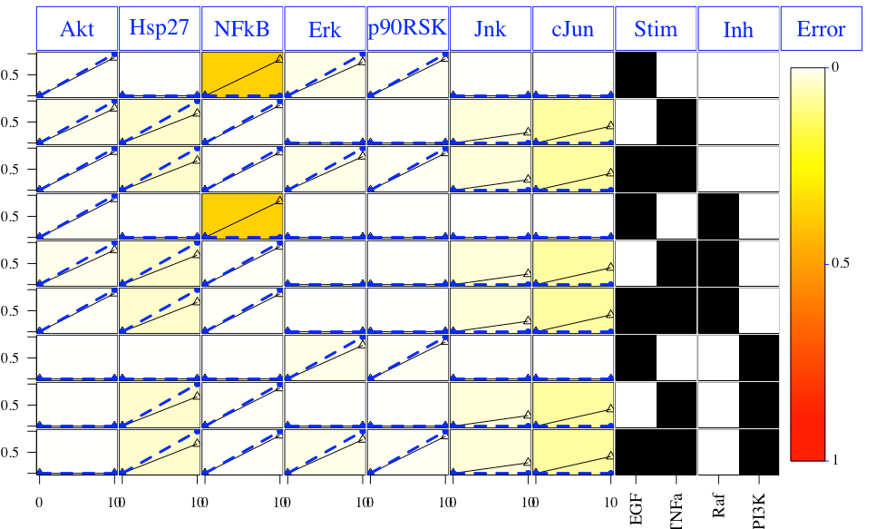
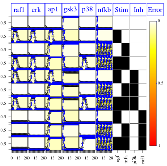
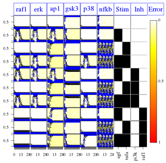
Finally, the following plot shows that errors across conditions and readouts are all small (white) by using this code:
cutAndPlotResultsDT(CNOlist=cnolist, model=model, upperB=upperB,
    lowerB=lowerB, bString=opt1$bString,    boolUpdates=boolUpdates)
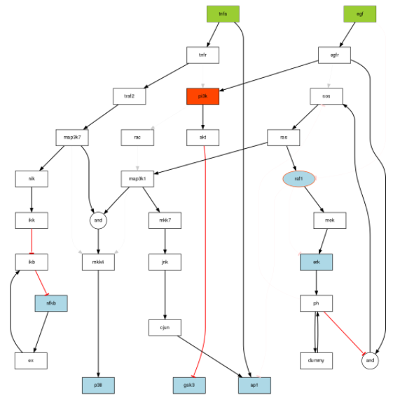
We then use the original True model stored in the SBMLqual (image on top) but alter it in the following ways:
The PKN is in SIF format available here 2013/sbml/PKN_noask1.sif
For the optimization, first we can check indeed that the True model can be used as a PKN to be optimised against the data generated. In theory, the final model should be identical to the True model.
pknmodel2 = readSIF("PKN_noask1.sif")
model = preprocessing(cnolist, pknmodel2, compression=F, expansion=T)
plotModel(model, cnolist)

# let us try this one where the additional links
# TNFR->PI3K and PI3K-RAC-Mapk31 are off as well as the unneeded AND and OR
gates.

# If you run the optimisation long enough, you'll get the optimised model to
# have the following bitstring:
optbs = c(1,1,1,1,1,1,1,1,1,1,1,1,1,1,1,1,1,1,1,1,1,1,1,0,0,0,0,1,1,1,0,0,0,1,0,0,0,1,0)

# It gives an RMSE = 0.031

opt1 = gaBinaryDT(CNOlist=cnolist, model=model,
    initBstring=optbs,boolUpdates=boolUpdates,maxTime=1000, lowerB=lowerB,
    upperB=upperB, stallGenMax=200, elitism=2, popSize=100, sizeFac=1e-4)
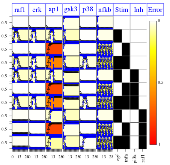
Finally, the following plot shows that errors across conditions and readouts are all small (white) by using this code:
cutAndPlotResultsDT(CNOlist=cnolist, model=model, upperB=upperB,
    lowerB=lowerB, bString=optbs,    boolUpdates=boolUpdates)
The fit is not good for the AP1 species. It means that
However, We can fix the issue of the missing link by using the CNORfeeder package to infer missing links based on the data solely.:
#
library(CNORfeeder)
pknmodel = readSIF("PKN_noask1.sif")
model = preprocessing(cnolist, pknmodel, compression=F, expansion=T)
# find new links
BTable = makeBTables(CNOlist=cnolist, k=2, measErr=c(0.1,0))
modelIntegr = mapBTables2model(BTable=BTable, model=model, allInter=F, compressed=FALSE)
modelIntegr$reacID[modelIntegr$indexIntegr]
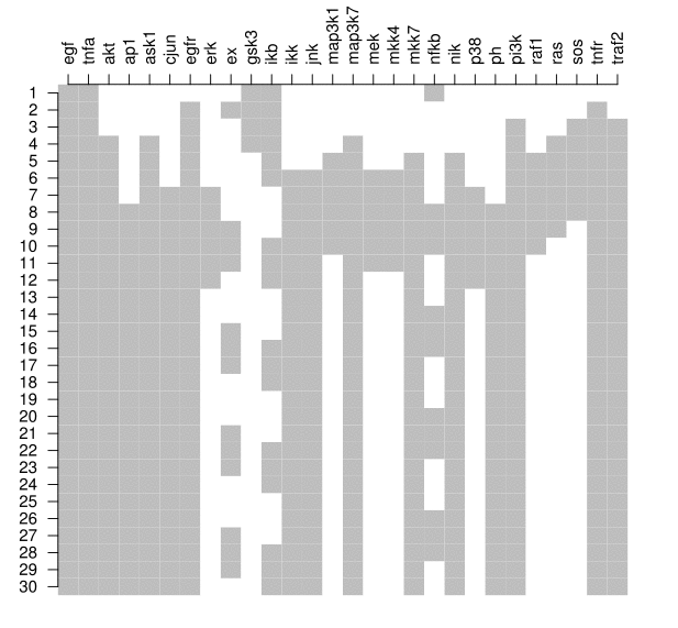
plotModel(model=modelIntegr, CNOlist=cnolist, indexIntegr=modelIntegr$indexIntegr)
You can see here below, in purple, the links that have been inferred.
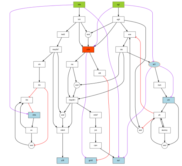
There is a proposed link between TNFa and ap1. This is related to the missing link we are looking for.
Does it improve the optimisation ?
# We could run the optimisation, which takes a while. The following
# bitstring is the optimal one
optbs_feeder = c(1, 1, 1, 1, 1, 1, 1, 1, 1, 1, 1, 1, 1, 1, 1, 1, 1, 1, 1, 1, 1, 1, 1, 0, 0, 0, 0, 1, 1, 1, 0, 0, 0, 1, 0, 1, 0, 1, 0, 1)

# we can check this hypothesis by using it as the initial guess:
opt1 = gaBinaryDT(CNOlist=cnolist, model=modelIntegr, boolUpdates=boolUpdates,maxTime=1000, lowerB=lowerB, upperB=upperB,
     stallGenMax=20, elitism=4, popSize=50, sizeFac=1e-4, initBstring=optbs_feeder)

# and check the final model
plotModel(modelIntegr, cnolist, bString=optbs_feeder)
One can check with the CNORdt optimisation that the new MSE is down to 0.00148 as compared to 0.031. The RMSE obtained is equivalent to the one obtained with hte True model (0.00142). The difference is due to the data being generated with a pure ODE formalism and the discrete time being used for the optimisation. We can check on the fitness plot that AP1 is now optimised properly:
cutAndPlotResultsDT(CNOlist=cnolist, model=modelIntegr, upperB=upperB,
    lowerB=lowerB, bString=optbs_feeder,    boolUpdates=boolUpdates)
So, the CNORfeeder analysis tells us that there is a missing link between TNFa stimulus and AP1 readouts. We know from the PKN that indeed there is a cross talk via ASK1 species. Without that knowledge, one can use different resources (e.g., intact) to figure out existing interactions between TNFa and ap1.
Other examples can be found on the documentation packages of CellnoptR, CNORdt, CNORfeder, CNORfuzzy, CNORode in bioconductor.