DOT: A flexible multi-objective optimization framework for transferring features across single-cell and spatial omics

Setup

# dot
library(DOT)

# for plotting
library(ggplot2)

The following example illustrates how DOT is used for inferring cell type composition of spots in a synthetic multicell spatial data of the primary motor cortex region (MOp) of the mouse brain. The reference single-cell RNA seq sample comes from a similar region and contains 44 cell types. Both spatial and single-cell data are down-sampled to 500 genes in this example.

data(dot.sample)

# gene x cell
dim(dot.sample$ref$counts)
#> [1]   500 20385

ggplot(as.data.frame(sort(table(dot.sample$ref$labels), decreasing = T)), aes(x = Var1, y = Freq))+
  geom_bar(stat="identity", fill="steelblue")+
  xlab("")+ylab("")+theme_bw()+
  theme(panel.background = element_rect(fill = 'white'), 
        panel.grid = element_blank(),
        axis.text.x = element_text(angle = 90, vjust = 0.5, hjust=1))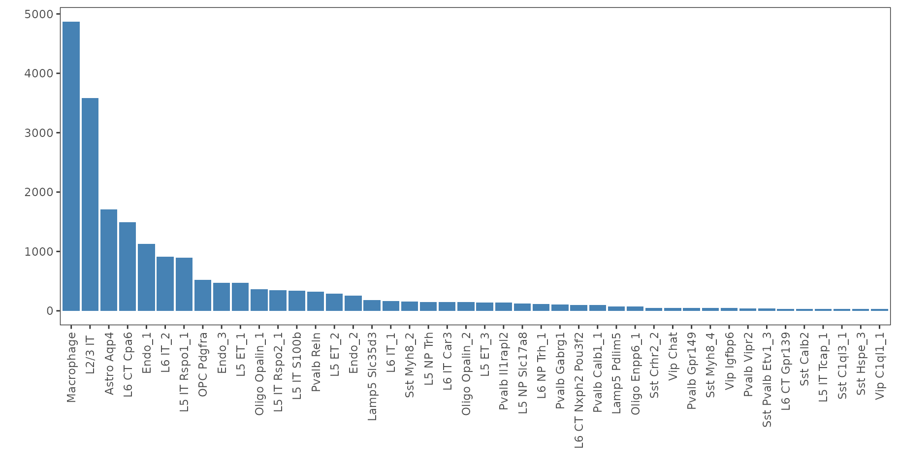

# gene x spot
dim(dot.sample$srt$counts)
#> [1] 500 361

plot_data <- dot.sample$srt$coordinates
ggplot(plot_data, aes(x = Col, y = Row))+
  geom_point(size = 5)+
  theme_bw()+
  theme(panel.background = element_rect(fill = 'white'), 
        panel.grid = element_blank(),
        axis.text = element_blank(), 
        axis.title = element_blank(), 
        axis.ticks = element_blank())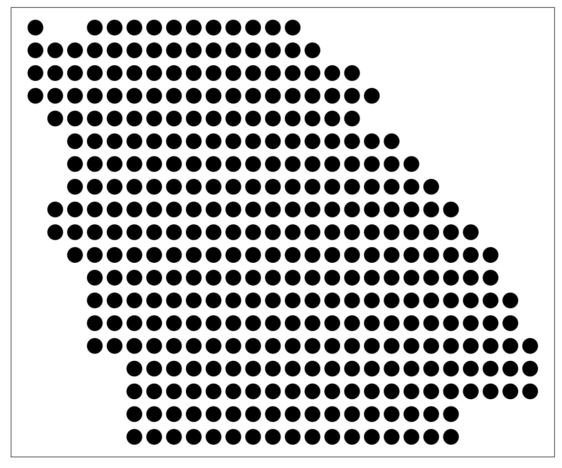

Decomposition

The first step of DOT is to set up a DOT object. DOT takes two main inputs:

ref_data is either a matrix, dgMatrix, or data.frame or a Seurat/anndata object containing the gene x cell count matrix for the reference single-cell data.
If ref_data is a matrix, dgMatrix, or data.frame, then ref_annotations must be supplied as a 1-dimensional vector of cell annotations.
If ref_data is a Seurat or an anndata object, then ref_annotations can be either a 1-dimensional vector of cell annotations, a character indicating the ident/obs contained therein, or can be NULL in which case annotations are extracted from the object.
srt_data is likewise either a matrix, dgMatrix, or data.frame or a Seurat/anndata object containing the gene x spot/cell count matrix for the target spatial data.
If srt_data is a matrix, dgMatrix, or data.frame, then srt_coords must be supplied as a 2 x spot matrix of locations.
If srt_data is a Seurat or an anndata object, then srt_coords can be either 2 x spot matrix of locations or can be NULL in which case locations are extracted from the object.

In the following example, we supply the count matrices as dgMatrix objects and supply the annotations/locations explicitly.

dot.srt <- setup.srt(srt_data = dot.sample$srt$counts, srt_coords = dot.sample$srt$coordinates)
dot.ref <- setup.ref(ref_data = dot.sample$ref$counts, ref_annotations = dot.sample$ref$labels, 10)

dot <- create.DOT(dot.srt, dot.ref)

We are now ready to perform decomposition:

dot <- run.DOT.lowresolution(dot,  # The DOT object created above
                             ratios_weight = 0,       # Abundance weight; a larger value more closely matches the abundance of cell types in the spatial data to those in the reference data
                             max_spot_size = 20, # Maximum size of spots (20 is usually sufficiently large for Visium slides) 
                             verbose = FALSE)

dim(dot@weights)
#> [1] 361  44

Plotting

The output of DOT is contained in dot@weights which has spots as rows and cell types as columns, with each row denoting the cell type composition of the respective spot. A simple way of illustrating the cell type map is to annotate the spots based on the label of the most likely cell type.

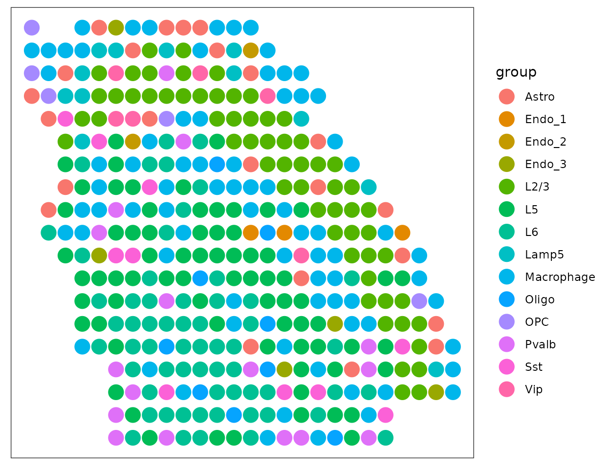
Cell type map at the given annotation level:

plot_data <- dot.sample$srt$coordinates
plot_data$celltype <- colnames(dot@weights)[apply(dot@weights, 1, which.max)]
ggplot(plot_data, aes(x = Col, y = Row, color = celltype))+
  geom_point(size = 5)+
  theme_bw()+
  theme(panel.background = element_rect(fill = 'white'), 
        panel.grid = element_blank(),
        axis.text = element_blank(), 
        axis.title = element_blank(), 
        axis.ticks = element_blank())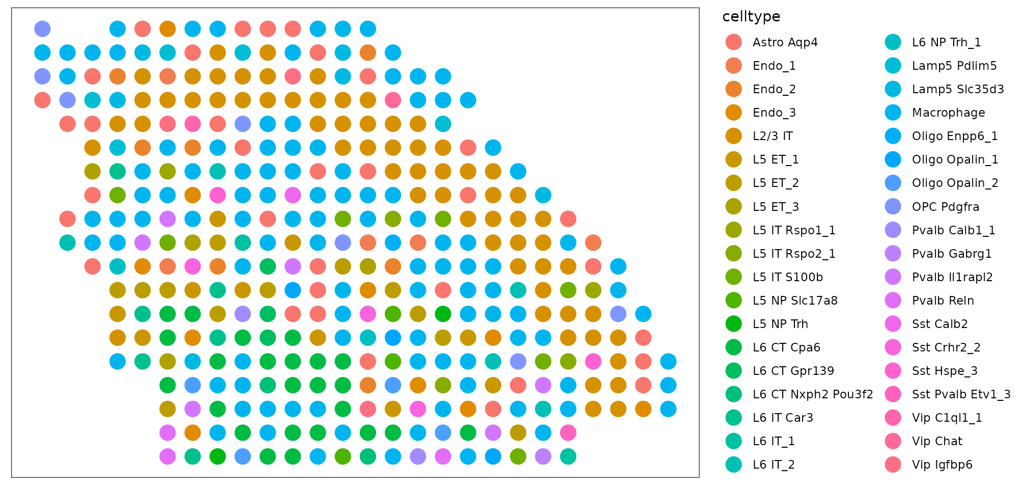

Cell type map at a higher annotation level:

groups <- sapply(colnames(dot@weights), function(x) stringr::str_split(x, " ")[[1]][1])
agg_weights <- t(rowsum(t(dot@weights), groups))
plot_data$group <- colnames(agg_weights)[apply(agg_weights, 1, which.max)]

ggplot(plot_data, aes(x = Col, y = Row, color = group))+
  geom_point(size = 5)+
  theme_bw()+
  theme(panel.background = element_rect(fill = 'white'), 
        panel.grid = element_blank(),
        axis.text = element_blank(), 
        axis.title = element_blank(), 
        axis.ticks = element_blank())

Arezou Rahimi

2024-04-26

Setup

Decomposition

Plotting