Context-specific metabolic networks from omics#
Here we will illustrate the use of the iMAT method, as implemented in CORNETO, to extract context specific metabolic networks from transcriptomics. CORNETO implements an extension of iMAT to support multiple samples, and also gives more control for customization.
We will use the core E. coli PKN, and microarray-based gene expression data corresponding to a anaerobic growth on glucose of a wild-type E. coli strain. This tutorial is based on the original COBRA tutorial.
import corneto as cn
import pandas as pd
import numpy as np

cn.info()

|
|
from corneto.methods.future.imat import MultiSampleIMAT

MultiSampleIMAT.show_citations()
---------------------------------------------------------------------------
AttributeError                            Traceback (most recent call last)
Cell In[2], line 3
      1 from corneto.methods.future.imat import MultiSampleIMAT
----> 3 MultiSampleIMAT.show_citations()

AttributeError: type object 'MultiSampleIMAT' has no attribute 'show_citations'
Loading data from COBRA#
We will use the ecoli core metabolic network and ecoli data example obtained from the COBRA package. This dataset contains 4 biological replicates. In this tutorial, we will use the single sample iMAT, we will average the expression and use this for analysis, since we are not interesed in analysing differences of the replicates
from corneto.io import import_cobra_model

G = import_cobra_model("../../tests/gem/ecoli_core.zip")
df_expr = pd.read_csv("../../tests/gem/ecoli_example_data.zip")
df_expr
| gene | raw_value_1 | raw_value_2 | raw_value_3 | raw_value_4 | value | |
|---|---|---|---|---|---|---|
| 0 | b0008 | 11.211265 | 12.030984 | 12.017371 | 11.674179 | 11.733450 |
| 1 | b0114 | 11.767118 | 11.581649 | 11.885833 | 11.571045 | 11.701411 |
| 2 | b0115 | 11.020531 | 10.813589 | 11.144573 | 11.362138 | 11.085208 |
| 3 | b0116 | 10.299068 | 10.562963 | 10.788094 | 10.425459 | 10.518896 |
| 4 | b0118 | 6.116122 | 6.437554 | 6.956686 | 6.229419 | 6.434945 |
| ... | ... | ... | ... | ... | ... | ... |
| 131 | b4153 | 9.647255 | 10.089110 | 8.685851 | 8.902372 | 9.331147 |
| 132 | b4154 | 9.176739 | 9.387545 | 8.841818 | 8.510611 | 8.979178 |
| 133 | b4232 | 9.490210 | 9.201019 | 9.321175 | 9.235511 | 9.311979 |
| 134 | b4301 | 2.335597 | 2.338372 | 2.317967 | 2.270161 | 2.315524 |
| 135 | b4395 | 2.431005 | 2.827751 | 2.822822 | 2.825172 | 2.726687 |
136 rows × 6 columns
G.shape
(77, 91)
# We can inspect the content of the network
G.get_attr_edges()[:5]
[{'__edge_type': 'directed',
  'id': 'EX_ac_b',
  '__source_attr': {'ac_b': {'__value': -1.0}},
  '__target_attr': {},
  'default_lb': -1000.0,
  'default_ub': 1000.0,
  'GPR': ''},
 {'__edge_type': 'directed',
  'id': 'EX_akg_b',
  '__source_attr': {'akg_b': {'__value': -1.0}},
  '__target_attr': {},
  'default_lb': -1000.0,
  'default_ub': 1000.0,
  'GPR': ''},
 {'__edge_type': 'directed',
  'id': 'EX_co2_b',
  '__source_attr': {'co2_b': {'__value': -1.0}},
  '__target_attr': {},
  'default_lb': -1000.0,
  'default_ub': 1000.0,
  'GPR': ''},
 {'__edge_type': 'directed',
  'id': 'EX_etoh_b',
  '__source_attr': {'etoh_b': {'__value': -1.0}},
  '__target_attr': {},
  'default_lb': -1000.0,
  'default_ub': 1000.0,
  'GPR': ''},
 {'__edge_type': 'directed',
  'id': 'EX_for_b',
  '__source_attr': {'for_b': {'__value': -1.0}},
  '__target_attr': {},
  'default_lb': -1000.0,
  'default_ub': 1000.0,
  'GPR': ''}]
Mapping data using Gene-Protein-Reaction (GPR) rules#
We need to compute reaction scores from gene expression data. For this, we will classify genes as highly expressed and lowly expressed based on thresholds applied to the marginal distribution of gene intensities. Then, we will map these values by applying the Gene-Protein-Reaction (GPR) rules included in the Ecoli PKN.
from corneto.methods.metabolism import evaluate_gpr_expression, get_unique_genes

genes = get_unique_genes(G, startswith="b")
len(genes)
101
df_expr.set_index("gene").stack().to_frame(name='expression').hist(bins=30);
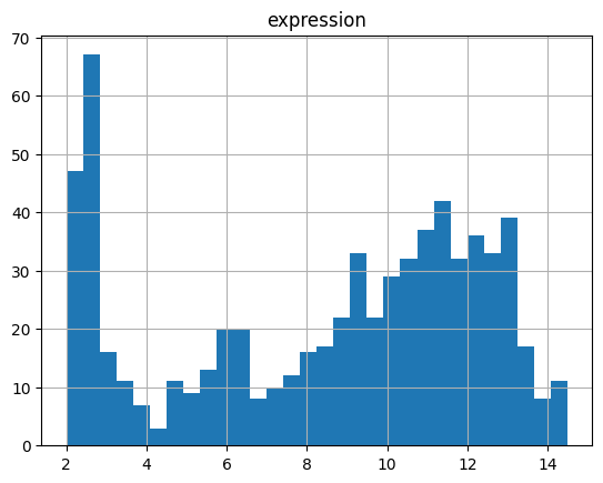
df_expr["high"] = (df_expr["value"] >= 8).astype(int)
df_expr["low"] = (df_expr["value"] <= 4).astype(int)
df_expr["score"] = df_expr["high"] - df_expr["low"]
df_expr
| gene | raw_value_1 | raw_value_2 | raw_value_3 | raw_value_4 | value | high | low | score | |
|---|---|---|---|---|---|---|---|---|---|
| 0 | b0008 | 11.211265 | 12.030984 | 12.017371 | 11.674179 | 11.733450 | 1 | 0 | 1 |
| 1 | b0114 | 11.767118 | 11.581649 | 11.885833 | 11.571045 | 11.701411 | 1 | 0 | 1 |
| 2 | b0115 | 11.020531 | 10.813589 | 11.144573 | 11.362138 | 11.085208 | 1 | 0 | 1 |
| 3 | b0116 | 10.299068 | 10.562963 | 10.788094 | 10.425459 | 10.518896 | 1 | 0 | 1 |
| 4 | b0118 | 6.116122 | 6.437554 | 6.956686 | 6.229419 | 6.434945 | 0 | 0 | 0 |
| ... | ... | ... | ... | ... | ... | ... | ... | ... | ... |
| 131 | b4153 | 9.647255 | 10.089110 | 8.685851 | 8.902372 | 9.331147 | 1 | 0 | 1 |
| 132 | b4154 | 9.176739 | 9.387545 | 8.841818 | 8.510611 | 8.979178 | 1 | 0 | 1 |
| 133 | b4232 | 9.490210 | 9.201019 | 9.321175 | 9.235511 | 9.311979 | 1 | 0 | 1 |
| 134 | b4301 | 2.335597 | 2.338372 | 2.317967 | 2.270161 | 2.315524 | 0 | 1 | -1 |
| 135 | b4395 | 2.431005 | 2.827751 | 2.822822 | 2.825172 | 2.726687 | 0 | 1 | -1 |
136 rows × 9 columns
values = df_expr[["gene", "score"]].set_index("gene").to_dict()["score"]
e = evaluate_gpr_expression(G.get_attr_from_edges("GPR"), values)
pd.DataFrame({"id": G.get_attr_from_edges("id"), "score": e})
| id | score | |
|---|---|---|
| 0 | EX_ac_b | 0 |
| 1 | EX_akg_b | 0 |
| 2 | EX_co2_b | 0 |
| 3 | EX_etoh_b | 0 |
| 4 | EX_for_b | 0 |
| ... | ... | ... |
| 86 | TALA | 1 |
| 87 | THD2 | 1 |
| 88 | TKT1 | 1 |
| 89 | TKT2 | 1 |
| 90 | TPI | 1 |
91 rows × 2 columns
Context-specific network inference#
We will use the reaction scores to create a Data object. The id corresponds to the reaction id of the PKN, and the value to the reaction score. We indicate that these features map to edges (reactions) with mapping = edge. Note that if mapping = none, then it will be assumed that the dataset contains genes, and automatic GPR will be performed to translate from genes to reaction scores.
# Create a dataset (here we only have 1 sample, which is the mean of the four measurements)
from corneto._data import Data

feats = dict()
for edge, val in zip(G.get_attr_from_edges("id"), e):
    feats[edge] = {"value": val, "mapping": "edge"}
data = {
    "sample1": feats
}
data = Data.from_cdict(data)
data
Data(n_samples=1, n_feats=[91])
We run the iMAT method (in this case, only 1 sample, which is the mean of the 4 biological replicates)
# eps is the min absolute flux value that we will consider
# for reactions with positive scores, i.e., if a reaction
# with a positive score is included in the context specific
# metabolic network, it has to be able to carry an absolute
# metabolic flux value above eps.
eps = 1e-2

# We will also add a small penalty to make networks sparser.
# When we have more than 1 sample, this parameter controls
# the regularization across samples, blocking entire groups
# of reactions across samples. Here, we are just penalizing
# the inclusion of reactions not needed to fit the reaction
# scores
m = MultiSampleIMAT(lambda_reg=1e-3, eps=eps)
P = m.build(G, data)
P.expr
{'_flow': _flow: Variable((91,), _flow),
 '_flow_ipos': _flow_ipos: Variable((91,), _flow_ipos, boolean=True),
 '_flow_ineg': _flow_ineg: Variable((91,), _flow_ineg, boolean=True),
 'edge_has_flux': edge_has_flux: Variable((91,), edge_has_flux, boolean=True),
 'flow': _flow: Variable((91,), _flow)}
P.solve(solver="scipy", verbosity=0);
The final result indicates that 1 reaction with positive score was not selected, and 1 reaction with negative score was included. In total, the network contains 61 reactions with fluxes. The last value corresponds to the number of reactions that were not blocked.
for o in P.objectives:
    print(o.value)
1.0
1.0
61.0
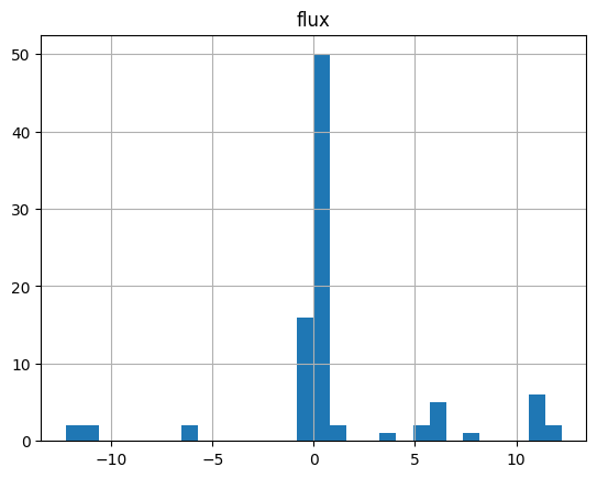
# Metabolic fluxes correspond to values of the flow variable
# Note that there are 91 values, corresponding to the 91 reactions
# in the PKN

df_sol = pd.DataFrame(
    P.expr.flow.value, index=G.get_attr_from_edges("id"), columns=["flux"]
)
df_sol
| flux | |
|---|---|
| EX_ac_b | 5.226570e-02 |
| EX_akg_b | -5.204170e-18 |
| EX_co2_b | 1.108361e+01 |
| EX_etoh_b | 1.123012e+01 |
| EX_for_b | 4.553438e-01 |
| ... | ... |
| TALA | -1.000000e-02 |
| THD2 | 5.008158e+00 |
| TKT1 | -1.000000e-02 |
| TKT2 | -3.690516e-02 |
| TPI | 6.141758e+00 |
91 rows × 1 columns
df_sol.hist(bins=30)
array([[<Axes: title={'center': 'flux'}>]], dtype=object)
selected_reactions = df_sol[df_sol.flux.abs() >= eps*(1-eps)].index.values.tolist()
len(selected_reactions)
61
np.sum(P.expr.edge_has_flux.value)
61.0
# Extract the context specific network
G_ctx = G.edge_subgraph(np.flatnonzero(P.expr.edge_has_flux.value))
G_ctx.shape
(57, 61)
G_ctx.plot(layout="neato")

Old version#
Original experiments in the manuscript used the old multicondition_imat:
from corneto.methods.metabolism.fba import multicondition_imat

P = multicondition_imat(G, np.array(e), alpha=1e-3, eps=eps)
P.solve(solver="scipy");
for o in P.objectives:
    print(o.value)
2.0
60.0
Citations#
MultiSampleIMAT.show_bibtex()