Single sample intracellular signalling network inference#
In this notebook we showcase how to use the advanced CARNIVAL implementation available in CORNETO. This implementation extends the capabilities of the original CARNIVAL method by enabling advanced modelling and injection of knowledge for hypothesis generation. We will use a dataset consisting of 6 samples of hepatic stellate cells (HSC) where three of them were activated by the cytokine Transforming growth factor (TGF-β).
In the first part, we will show how to estimate Transcription Factor activities from gene expression data, following the Decoupler tutorial for functional analysis. Then, we will use the CARNIVAL method available in CORNETO to infer a network from TFs to receptors, assuming that we don’t really know which treatment was used.
# --- Saezlab tools ---
# https://decoupler-py.readthedocs.io/
import gzip
import os
import shutil
import tempfile
import urllib.request

import decoupler as dc
import numpy as np

# https://omnipathdb.org/
import omnipath as op

# Additional packages
import pandas as pd

# --- Additional libs ---
# Pydeseq for differential expression analysis
from pydeseq2.dds import DefaultInference, DeseqDataSet
from pydeseq2.ds import DeseqStats

# https://saezlab.github.io/
import corneto as cn
max_time = 300
seed = 0
# We need to download the dataset, available at GEO GSE151251
url = "https://www.ncbi.nlm.nih.gov/geo/download/?acc=GSE151251&format=file&file=GSE151251%5FHSCs%5FCtrl%2Evs%2EHSCs%5FTGFb%2Ecounts%2Etsv%2Egz"

adata = None
with tempfile.TemporaryDirectory() as tmpdirname:
    # Path for the gzipped file in the temp folder
    gz_file_path = os.path.join(tmpdirname, "counts.txt.gz")

    # Download the file
    with urllib.request.urlopen(url) as response:
        with open(gz_file_path, "wb") as out_file:
            shutil.copyfileobj(response, out_file)

    # Decompress the file
    decompressed_file_path = gz_file_path[:-3]  # Removing '.gz' extension
    with gzip.open(gz_file_path, "rb") as f_in:
        with open(decompressed_file_path, "wb") as f_out:
            shutil.copyfileobj(f_in, f_out)

    adata = pd.read_csv(decompressed_file_path, index_col=2, sep="\t").iloc[:, 5:].T

adata
| GeneName | DDX11L1 | WASH7P | MIR6859-1 | MIR1302-11 | MIR1302-9 | FAM138A | OR4G4P | OR4G11P | OR4F5 | RP11-34P13.7 | ... | MT-ND4 | MT-TH | MT-TS2 | MT-TL2 | MT-ND5 | MT-ND6 | MT-TE | MT-CYB | MT-TT | MT-TP |
|---|---|---|---|---|---|---|---|---|---|---|---|---|---|---|---|---|---|---|---|---|---|
| 25_HSCs-Ctrl1 | 0 | 9 | 10 | 1 | 0 | 0 | 0 | 0 | 0 | 33 | ... | 93192 | 342 | 476 | 493 | 54466 | 17184 | 1302 | 54099 | 258 | 475 |
| 26_HSCs-Ctrl2 | 0 | 12 | 14 | 0 | 0 | 0 | 0 | 0 | 0 | 66 | ... | 114914 | 355 | 388 | 436 | 64698 | 21106 | 1492 | 62679 | 253 | 396 |
| 27_HSCs-Ctrl3 | 0 | 14 | 10 | 0 | 0 | 0 | 0 | 0 | 0 | 52 | ... | 155365 | 377 | 438 | 480 | 85650 | 31860 | 2033 | 89559 | 282 | 448 |
| 31_HSCs-TGFb1 | 0 | 11 | 16 | 0 | 0 | 0 | 0 | 0 | 0 | 54 | ... | 110866 | 373 | 441 | 481 | 60325 | 19496 | 1447 | 66283 | 172 | 341 |
| 32_HSCs-TGFb2 | 0 | 5 | 8 | 0 | 0 | 0 | 0 | 0 | 0 | 44 | ... | 45488 | 239 | 331 | 343 | 27442 | 9054 | 624 | 27535 | 96 | 216 |
| 33_HSCs-TGFb3 | 0 | 12 | 5 | 0 | 0 | 0 | 0 | 0 | 0 | 32 | ... | 70704 | 344 | 453 | 497 | 45443 | 13796 | 1077 | 43415 | 192 | 243 |
6 rows × 64253 columns
Data preprocessing#
We will use AnnData and PyDeseq2 to pre-process the data and compute differential expression between control and tretament
from anndata import AnnData

adata = AnnData(adata, dtype=np.float32)
adata.var_names_make_unique()
adata
AnnData object with n_obs × n_vars = 6 × 64253
# Process treatment information
adata.obs["condition"] = [
    "control" if "-Ctrl" in sample_id else "treatment" for sample_id in adata.obs.index
]

# Process sample information
adata.obs["sample_id"] = [sample_id.split("_")[0] for sample_id in adata.obs.index]

# Visualize metadata
adata.obs
| condition | sample_id | |
|---|---|---|
| 25_HSCs-Ctrl1 | control | 25 |
| 26_HSCs-Ctrl2 | control | 26 |
| 27_HSCs-Ctrl3 | control | 27 |
| 31_HSCs-TGFb1 | treatment | 31 |
| 32_HSCs-TGFb2 | treatment | 32 |
| 33_HSCs-TGFb3 | treatment | 33 |
# Obtain genes that pass the thresholds
genes = dc.filter_by_expr(
    adata, group="condition", min_count=10, min_total_count=15, large_n=1, min_prop=1
)

# Filter by these genes
adata = adata[:, genes].copy()
adata
AnnData object with n_obs × n_vars = 6 × 19713
    obs: 'condition', 'sample_id'
# Estimation of differential expression

inference = DefaultInference()
dds = DeseqDataSet(
    adata=adata,
    design_factors="condition",
    refit_cooks=True,
    inference=inference,
)
# Compute LFCs
dds.deseq2()
Using None as control genes, passed at DeseqDataSet initialization
stat_res = DeseqStats(
    dds, contrast=["condition", "treatment", "control"], inference=inference
)

stat_res.summary()
Log2 fold change & Wald test p-value: condition treatment vs control
                  baseMean  log2FoldChange     lfcSE      stat    pvalue  \
GeneName
WASH7P           10.349784       -0.011139  0.651659 -0.017093  0.986362
MIR6859-1        10.114621        0.000646  0.657316  0.000982  0.999216
RP11-34P13.7     45.731312        0.078207  0.324393  0.241087  0.809487
RP11-34P13.8     29.498379       -0.065184  0.393560 -0.165626  0.868451
CICP27          106.032659        0.150600  0.222955  0.675471  0.499377
...                    ...             ...       ...       ...       ...
MT-ND6        17914.984474       -0.435304  0.278796 -1.561372  0.118436
MT-TE          1281.293477       -0.332495  0.288073 -1.154204  0.248416
MT-CYB        54955.449372       -0.313285  0.286900 -1.091966  0.274848
MT-TT           204.692221       -0.485883  0.220564 -2.202915  0.027601
MT-TP           345.049755       -0.460674  0.161681 -2.849280  0.004382

                  padj
GeneName
WASH7P        0.991392
MIR6859-1     0.999509
RP11-34P13.7  0.877264
RP11-34P13.8  0.917051
CICP27        0.637262
...                ...
MT-ND6        0.210925
MT-TE         0.380027
MT-CYB        0.411208
MT-TT         0.061573
MT-TP         0.012206

[19713 rows x 6 columns]
results_df = stat_res.results_df
results_df
| baseMean | log2FoldChange | lfcSE | stat | pvalue | padj | |
|---|---|---|---|---|---|---|
| GeneName | ||||||
| WASH7P | 10.349784 | -0.011139 | 0.651659 | -0.017093 | 0.986362 | 0.991392 |
| MIR6859-1 | 10.114621 | 0.000646 | 0.657316 | 0.000982 | 0.999216 | 0.999509 |
| RP11-34P13.7 | 45.731312 | 0.078207 | 0.324393 | 0.241087 | 0.809487 | 0.877264 |
| RP11-34P13.8 | 29.498379 | -0.065184 | 0.393560 | -0.165626 | 0.868451 | 0.917051 |
| CICP27 | 106.032659 | 0.150600 | 0.222955 | 0.675471 | 0.499377 | 0.637262 |
| ... | ... | ... | ... | ... | ... | ... |
| MT-ND6 | 17914.984474 | -0.435304 | 0.278796 | -1.561372 | 0.118436 | 0.210925 |
| MT-TE | 1281.293477 | -0.332495 | 0.288073 | -1.154204 | 0.248416 | 0.380027 |
| MT-CYB | 54955.449372 | -0.313285 | 0.286900 | -1.091966 | 0.274848 | 0.411208 |
| MT-TT | 204.692221 | -0.485883 | 0.220564 | -2.202915 | 0.027601 | 0.061573 |
| MT-TP | 345.049755 | -0.460674 | 0.161681 | -2.849280 | 0.004382 | 0.012206 |
19713 rows × 6 columns
Prior knowledge with Decoupler and Omnipath#
# Retrieve CollecTRI gene regulatory network (through Omnipath)
collectri = dc.get_collectri(organism="human", split_complexes=False)
collectri
| source | target | weight | PMID | |
|---|---|---|---|---|
| 0 | MYC | TERT | 1 | 10022128;10491298;10606235;10637317;10723141;1... |
| 1 | SPI1 | BGLAP | 1 | 10022617 |
| 2 | SMAD3 | JUN | 1 | 10022869;12374795 |
| 3 | SMAD4 | JUN | 1 | 10022869;12374795 |
| 4 | STAT5A | IL2 | 1 | 10022878;11435608;17182565;17911616;22854263;2... |
| ... | ... | ... | ... | ... |
| 43173 | NFKB | hsa-miR-143-3p | 1 | 19472311 |
| 43174 | AP1 | hsa-miR-206 | 1 | 19721712 |
| 43175 | NFKB | hsa-miR-21-5p | 1 | 20813833;22387281 |
| 43176 | NFKB | hsa-miR-224-5p | 1 | 23474441;23988648 |
| 43177 | AP1 | hsa-miR-144 | 1 | 23546882 |
43178 rows × 4 columns
mat = results_df[["stat"]].T.rename(index={"stat": "treatment.vs.control"})
mat
| GeneName | WASH7P | MIR6859-1 | RP11-34P13.7 | RP11-34P13.8 | CICP27 | FO538757.2 | AP006222.2 | RP4-669L17.10 | MTND1P23 | MTND2P28 | ... | MT-ND4 | MT-TH | MT-TS2 | MT-TL2 | MT-ND5 | MT-ND6 | MT-TE | MT-CYB | MT-TT | MT-TP |
|---|---|---|---|---|---|---|---|---|---|---|---|---|---|---|---|---|---|---|---|---|---|
| treatment.vs.control | -0.017093 | 0.000982 | 0.241087 | -0.165626 | 0.675471 | -1.646005 | 2.042031 | -0.376975 | -1.994364 | -0.498507 | ... | -1.435973 | 0.75501 | 1.139089 | 1.167108 | -1.242582 | -1.561372 | -1.154204 | -1.091966 | -2.202915 | -2.84928 |
1 rows × 19713 columns
tf_acts, tf_pvals = dc.run_ulm(mat=mat, net=collectri, verbose=True)
tf_acts
Running ulm on mat with 1 samples and 19713 targets for 655 sources.
| ABL1 | AHR | AIRE | AP1 | APEX1 | AR | ARID1A | ARID3A | ARID3B | ARID4A | ... | ZNF362 | ZNF382 | ZNF384 | ZNF395 | ZNF436 | ZNF699 | ZNF76 | ZNF804A | ZNF91 | ZXDC | |
|---|---|---|---|---|---|---|---|---|---|---|---|---|---|---|---|---|---|---|---|---|---|
| treatment.vs.control | -2.179559 | -1.561975 | -1.822945 | -1.981524 | -2.67045 | 0.21549 | -3.931481 | 0.870412 | 1.648694 | -0.611922 | ... | -0.062613 | 2.121308 | 1.886897 | -1.14056 | -1.571203 | -1.276569 | -0.116815 | 3.373271 | 0.86042 | -2.742784 |
1 rows × 655 columns
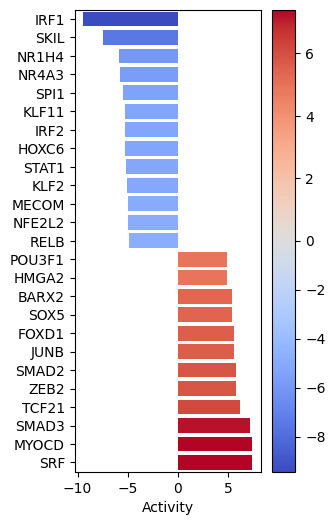
dc.plot_barplot(
    acts=tf_acts, contrast="treatment.vs.control", top=25, vertical=True, figsize=(3, 6)
)
# We obtain ligand-receptor interactions from Omnipath, and we keep only the receptors
# This is our list of a prior potential receptors from which we will infer the network
unique_receptors = set(
    op.interactions.LigRecExtra.get(genesymbols=True)[
        "target_genesymbol"
    ].values.tolist()
)
len(unique_receptors)
1201
df_de_receptors = results_df.loc[results_df.index.intersection(unique_receptors)]
df_de_receptors = df_de_receptors.sort_values(by="stat", ascending=False)
df_de_receptors.plot.scatter(x="log2FoldChange", y="stat")
<Axes: xlabel='log2FoldChange', ylabel='stat'>
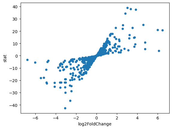
# We will take the top 20 receptors that increased the expression after treatment
df_top_receptors = df_de_receptors.head(20)
df_top_receptors
| baseMean | log2FoldChange | lfcSE | stat | pvalue | padj | |
|---|---|---|---|---|---|---|
| GeneName | ||||||
| CDH6 | 28262.296983 | 3.019806 | 0.077448 | 38.991476 | 0.000000e+00 | 0.000000e+00 |
| CRLF1 | 7919.672343 | 3.341645 | 0.088026 | 37.962070 | 0.000000e+00 | 0.000000e+00 |
| FZD8 | 2719.781498 | 3.843017 | 0.102718 | 37.413242 | 2.380145e-306 | 2.469463e-303 |
| CDH2 | 7111.507547 | 2.809462 | 0.081958 | 34.279439 | 1.589168e-257 | 9.213903e-255 |
| DYSF | 441.449511 | 4.593250 | 0.182196 | 25.210487 | 3.073961e-140 | 5.362566e-138 |
| INHBA | 24329.359641 | 2.598613 | 0.104350 | 24.902821 | 6.934669e-137 | 1.139193e-134 |
| CELSR1 | 492.324435 | 3.517315 | 0.154487 | 22.767746 | 9.574546e-115 | 1.258287e-112 |
| PDGFC | 5481.167075 | 1.894858 | 0.083837 | 22.601620 | 4.177614e-113 | 5.453862e-111 |
| VDR | 1450.304353 | 2.555008 | 0.116797 | 21.875720 | 4.424761e-106 | 5.286382e-104 |
| HHIP | 379.064034 | 6.005841 | 0.287363 | 20.899827 | 5.373904e-97 | 5.323406e-95 |
| IGF1 | 361.189076 | 6.462657 | 0.311785 | 20.727921 | 1.939904e-95 | 1.874575e-93 |
| NPTN | 12640.971164 | 1.418676 | 0.079385 | 17.870802 | 1.991103e-71 | 1.226582e-69 |
| EFNB2 | 3320.076805 | 1.560331 | 0.087871 | 17.757127 | 1.518082e-70 | 9.096034e-69 |
| ITGB3 | 6530.314159 | 1.364766 | 0.078800 | 17.319326 | 3.362752e-67 | 1.851674e-65 |
| TGFB1 | 8948.243694 | 1.335271 | 0.077647 | 17.196617 | 2.814963e-66 | 1.524488e-64 |
| IL21R | 259.221468 | 3.227903 | 0.192069 | 16.805944 | 2.207685e-63 | 1.130392e-61 |
| ITGA1 | 26223.832504 | 1.310351 | 0.079861 | 16.407981 | 1.676899e-60 | 8.023475e-59 |
| FAP | 7231.157483 | 1.750901 | 0.115214 | 15.196911 | 3.706936e-52 | 1.488286e-50 |
| EGF | 144.262044 | 3.733297 | 0.251588 | 14.838931 | 8.205292e-50 | 3.063465e-48 |
| ITGA11 | 12471.033668 | 3.673199 | 0.250314 | 14.674378 | 9.407359e-49 | 3.377910e-47 |
Inferring intracellular signalling network with CARNIVAL and CORNETO#
CORNETO is a unified framework for knowledge-driven network inference. It includes a very flexible implementation of CARNIVAL that expands its original capabilities. We will see how to use it under different assumptions to extract a network from a prior knowledge network and a set of potential receptors + our estimated TFs
cn.info()

|
|
from corneto.methods.future import CarnivalFlow

CarnivalFlow.show_citations()
- Pablo Rodriguez-Mier, Martin Garrido-Rodriguez, Attila Gabor, Julio Saez-Rodriguez. Unified knowledge-driven network inference from omics data. bioRxiv, pp. 10 (2024).
- Anika Liu, Panuwat Trairatphisan, Enio Gjerga, Athanasios Didangelos, Jonathan Barratt, Julio Saez-Rodriguez. From expression footprints to causal pathways: contextualizing large signaling networks with CARNIVAL. NPJ systems biology and applications, Vol. 5, No. 1, pp. 40 (2019).
# We get only interactions from SIGNOR http://signor.uniroma2.it/
pkn = op.interactions.OmniPath.get(databases=["SIGNOR"], genesymbols=True)
pkn = pkn[pkn.consensus_direction == True]
pkn.head()
| source | target | source_genesymbol | target_genesymbol | is_directed | is_stimulation | is_inhibition | consensus_direction | consensus_stimulation | consensus_inhibition | curation_effort | references | sources | n_sources | n_primary_sources | n_references | references_stripped | |
|---|---|---|---|---|---|---|---|---|---|---|---|---|---|---|---|---|---|
| 0 | Q13976 | Q13507 | PRKG1 | TRPC3 | True | False | True | True | False | True | 9 | HPRD:14983059;KEA:14983059;ProtMapper:14983059... | HPRD;HPRD_KEA;HPRD_MIMP;KEA;MIMP;PhosphoPoint;... | 15 | 8 | 2 | 14983059;16331690 |
| 1 | Q13976 | Q9HCX4 | PRKG1 | TRPC7 | True | True | False | True | True | False | 3 | SIGNOR:21402151;TRIP:21402151;iPTMnet:21402151 | SIGNOR;TRIP;iPTMnet | 3 | 3 | 1 | 21402151 |
| 2 | Q13438 | Q9HBA0 | OS9 | TRPV4 | True | True | True | True | True | True | 3 | HPRD:17932042;SIGNOR:17932042;TRIP:17932042 | HPRD;SIGNOR;TRIP | 3 | 3 | 1 | 17932042 |
| 3 | P18031 | Q9H1D0 | PTPN1 | TRPV6 | True | False | True | True | False | True | 11 | DEPOD:15894168;DEPOD:17197020;HPRD:15894168;In... | DEPOD;HPRD;IntAct;Lit-BM-17;SIGNOR;SPIKE_LC;TRIP | 7 | 6 | 2 | 15894168;17197020 |
| 4 | P63244 | Q9BX84 | RACK1 | TRPM6 | True | False | True | True | False | True | 2 | SIGNOR:18258429;TRIP:18258429 | SIGNOR;TRIP | 2 | 2 | 1 | 18258429 |
pkn["interaction"] = pkn["is_stimulation"].astype(int) - pkn["is_inhibition"].astype(
    int
)
sel_pkn = pkn[["source_genesymbol", "interaction", "target_genesymbol"]]
sel_pkn
| source_genesymbol | interaction | target_genesymbol | |
|---|---|---|---|
| 0 | PRKG1 | -1 | TRPC3 |
| 1 | PRKG1 | 1 | TRPC7 |
| 2 | OS9 | 0 | TRPV4 |
| 3 | PTPN1 | -1 | TRPV6 |
| 4 | RACK1 | -1 | TRPM6 |
| ... | ... | ... | ... |
| 61542 | APC_PUF60_SIAH1_SKP1_TBL1X | -1 | CTNNB1 |
| 61543 | MAP2K6 | 1 | MAPK10 |
| 61544 | PRKAA1 | 1 | TP53 |
| 61545 | CNOT1_CNOT10_CNOT11_CNOT2_CNOT3_CNOT4_CNOT6_CN... | -1 | NANOS2 |
| 61546 | WNT16 | 1 | FZD3 |
60921 rows × 3 columns
# We create the CORNETO graph by importing the edges and interaction
from corneto.graph import Graph
from corneto.io import load_graph_from_sif_tuples
G = load_graph_from_sif_tuples(
    [(r[0], r[1], r[2]) for _, r in sel_pkn.iterrows() if r[1] != 0]
)
G.shape
(5442, 60034)
# As measurements, we take the estimated TFs, we will filter out TFs with p-val > 0.001
significant_tfs = (
    tf_acts[tf_pvals <= 0.001]
    .T.dropna()
    .sort_values(by="treatment.vs.control", ascending=False)
)
significant_tfs
| treatment.vs.control | |
|---|---|
| SRF | 7.402565 |
| MYOCD | 7.366407 |
| SMAD3 | 7.205507 |
| TCF21 | 6.178324 |
| ZEB2 | 5.804123 |
| ... | ... |
| SPI1 | -5.442575 |
| NR4A3 | -5.745412 |
| NR1H4 | -5.917429 |
| SKIL | -7.463470 |
| IRF1 | -9.437411 |
85 rows × 1 columns
# We keep only the ones in the PKN graph
measurements = significant_tfs.loc[significant_tfs.index.intersection(G.V)].to_dict()[
    "treatment.vs.control"
]
measurements
{'SRF': 7.402564525604248,
 'MYOCD': 7.36640739440918,
 'SMAD3': 7.205506801605225,
 'ZEB2': 5.8041229248046875,
 'SMAD2': 5.7937397956848145,
 'JUNB': 5.62872314453125,
 'HMGA2': 4.934858322143555,
 'POU3F1': 4.918986797332764,
 'RORA': 4.76252555847168,
 'SMAD4': 4.730061054229736,
 'MEF2A': 4.285721302032471,
 'FGF2': 4.222509860992432,
 'FOSL1': 3.9362800121307373,
 'SOX4': 3.92212176322937,
 'NCOA1': 3.8224685192108154,
 'ASXL1': 3.7563669681549072,
 'SFPQ': 3.7415316104888916,
 'FOSB': 3.7254574298858643,
 'SP7': 3.695308208465576,
 'CREB3': 3.6301043033599854,
 'NFATC3': 3.5302765369415283,
 'MEIS2': 3.4903156757354736,
 'ZNF804A': 3.3732707500457764,
 'TAL1': 3.353253126144409,
 'DLX5': 3.33522367477417,
 'DLX2': -3.2915139198303223,
 'CDX2': -3.296456813812256,
 'CEBPG': -3.307525396347046,
 'MAFA': -3.3084702491760254,
 'NFIB': -3.3599045276641846,
 'NFKB1': -3.4378252029418945,
 'RXRB': -3.4568121433258057,
 'STAT5A': -3.5282504558563232,
 'MSX2': -3.5356292724609375,
 'PLAGL1': -3.6181154251098633,
 'TP53': -3.6528894901275635,
 'GFI1': -3.6557135581970215,
 'NKX2-1': -3.6595804691314697,
 'MECP2': -3.7389347553253174,
 'CEBPA': -3.775284767150879,
 'CEBPB': -3.8758962154388428,
 'SMAD6': -3.8772501945495605,
 'WWTR1': -3.9811408519744873,
 'SMAD5': -4.017445087432861,
 'CIITA': -4.1478800773620605,
 'NFKBIB': -4.171163558959961,
 'PITX3': -4.213423728942871,
 'REL': -4.263958930969238,
 'IRF3': -4.2882513999938965,
 'PITX1': -4.355759620666504,
 'KLF8': -4.4818549156188965,
 'DNMT3A': -4.6564249992370605,
 'RELB': -4.845225811004639,
 'NFE2L2': -4.9314775466918945,
 'MECOM': -4.961089611053467,
 'STAT1': -5.2104878425598145,
 'HOXC6': -5.278722763061523,
 'IRF2': -5.287947177886963,
 'KLF11': -5.2895355224609375,
 'SPI1': -5.442574501037598,
 'NR4A3': -5.745412349700928,
 'NR1H4': -5.917429447174072,
 'SKIL': -7.463469505310059,
 'IRF1': -9.437411308288574}
# We will infer the direction, so for the inputs, we use a value of 0 (=unknown direction)
inputs = {k: 0 for k in df_top_receptors.index.intersection(G.V).values}
inputs
{'CDH6': 0,
 'CRLF1': 0,
 'FZD8': 0,
 'CDH2': 0,
 'INHBA': 0,
 'VDR': 0,
 'IGF1': 0,
 'EFNB2': 0,
 'ITGB3': 0,
 'TGFB1': 0,
 'IL21R': 0,
 'EGF': 0,
 'ITGA11': 0}
# Create the dataset in standard format
carnival_data = dict()
for inp, v in inputs.items():
    carnival_data[inp] = dict(value=v, role="input", mapping="vertex")
for out, v in measurements.items():
    carnival_data[out] = dict(value=v, role="output", mapping="vertex")
data = cn.Data.from_cdict({"sample1": carnival_data})
data
Data(n_samples=1, n_feats=[77])
carnival = CarnivalFlow(lambda_reg=0.5)
P = carnival.build(G, data)
P.expr
Unreachable vertices for sample: 0
{'edge_activates': edge_activates: Variable((3374, 1), edge_activates, boolean=True),
 'const0x1ed29ddbdc597523': const0x1ed29ddbdc597523: Constant(CONSTANT, NONNEGATIVE, (970, 3374)),
 '_flow': _flow: Variable((3374,), _flow),
 'edge_inhibits': edge_inhibits: Variable((3374, 1), edge_inhibits, boolean=True),
 'const0x70b316d8f961cc5': const0x70b316d8f961cc5: Constant(CONSTANT, NONNEGATIVE, (970, 3374)),
 '_dag_layer': _dag_layer: Variable((970, 1), _dag_layer),
 'flow': _flow: Variable((3374,), _flow),
 'vertex_value': Expression(AFFINE, UNKNOWN, (970, 1)),
 'vertex_activated': Expression(AFFINE, NONNEGATIVE, (970, 1)),
 'vertex_inhibited': Expression(AFFINE, NONNEGATIVE, (970, 1)),
 'edge_value': Expression(AFFINE, UNKNOWN, (3374, 1)),
 'edge_has_signal': Expression(AFFINE, NONNEGATIVE, (3374, 1))}
P.solve(solver="highs", max_seconds=60, verbosity=1);
===============================================================================
                                     CVXPY
                                     v1.6.4
===============================================================================
(CVXPY) Apr 16 11:41:50 AM: Your problem has 11092 variables, 31652 constraints, and 1 parameters.
(CVXPY) Apr 16 11:41:50 AM: It is compliant with the following grammars: DCP, DQCP
(CVXPY) Apr 16 11:41:50 AM: CVXPY will first compile your problem; then, it will invoke a numerical solver to obtain a solution.
(CVXPY) Apr 16 11:41:50 AM: Your problem is compiled with the CPP canonicalization backend.
-------------------------------------------------------------------------------
                                  Compilation
-------------------------------------------------------------------------------
(CVXPY) Apr 16 11:41:50 AM: Compiling problem (target solver=HIGHS).
(CVXPY) Apr 16 11:41:50 AM: Reduction chain: Dcp2Cone -> CvxAttr2Constr -> ConeMatrixStuffing -> HIGHS
(CVXPY) Apr 16 11:41:50 AM: Applying reduction Dcp2Cone
(CVXPY) Apr 16 11:41:50 AM: Applying reduction CvxAttr2Constr
(CVXPY) Apr 16 11:41:50 AM: Applying reduction ConeMatrixStuffing
(CVXPY) Apr 16 11:41:50 AM: Applying reduction HIGHS
(CVXPY) Apr 16 11:41:50 AM: Finished problem compilation (took 5.614e-02 seconds).
(CVXPY) Apr 16 11:41:50 AM: (Subsequent compilations of this problem, using the same arguments, should take less time.)
-------------------------------------------------------------------------------
                                Numerical solver
-------------------------------------------------------------------------------
(CVXPY) Apr 16 11:41:50 AM: Invoking solver HIGHS  to obtain a solution.
Running HiGHS 1.10.0 (git hash: fd86653): Copyright (c) 2025 HiGHS under MIT licence terms
MIP  has 31652 rows; 11092 cols; 111482 nonzeros; 6748 integer variables (6748 binary)
Coefficient ranges:
  Matrix [1e+00, 1e+03]
  Cost   [5e-01, 8e+00]
  Bound  [1e+00, 1e+00]
  RHS    [1e+00, 1e+03]
Presolving model
18338 rows, 10622 cols, 93928 nonzeros  0s
13396 rows, 9435 cols, 71834 nonzeros  0s
13024 rows, 9360 cols, 71388 nonzeros  0s

Solving MIP model with:
   13024 rows
   9360 cols (5850 binary, 0 integer, 0 implied int., 3510 continuous)
   71388 nonzeros

Src: B => Branching; C => Central rounding; F => Feasibility pump; H => Heuristic; L => Sub-MIP;
     P => Empty MIP; R => Randomized rounding; S => Solve LP; T => Evaluate node; U => Unbounded;
     z => Trivial zero; l => Trivial lower; u => Trivial upper; p => Trivial point; X => User solution

        Nodes      |    B&B Tree     |            Objective Bounds              |  Dynamic Constraints |       Work
Src  Proc. InQueue |  Leaves   Expl. | BestBound       BestSol              Gap |   Cuts   InLp Confl. | LpIters     Time

         0       0         0   0.00%   -298.7062635    inf                  inf        0      0      0         0     0.3s
         0       0         0   0.00%   -172.2083844    inf                  inf        0      0      5      1707     0.4s
 C       0       0         0   0.00%   -167.0036403    0                  Large      501     37     10      2237     1.2s
 L       0       0         0   0.00%   -166.1703069    -165.1703069       0.61%     1959    117     10      8802     3.9s

9.2% inactive integer columns, restarting
Model after restart has 12184 rows, 8682 cols (5196 bin., 0 int., 0 impl., 3486 cont.), and 63464 nonzeros

         0       0         0   0.00%   -166.1703069    -165.1703069       0.61%       44      0      0      9812     4.0s
         0       0         0   0.00%   -166.1703069    -165.1703069       0.61%       44     28      4     11329     4.1s

Symmetry detection completed in 0.0s
Found 29 generator(s)

         8       0         4 100.00%   -165.1703069    -165.1703069       0.00%      902     56     16     21107     7.1s

Solving report
  Status            Optimal
  Primal bound      -165.170306921
  Dual bound        -165.170306921
  Gap               0% (tolerance: 0.01%)
  P-D integral      0.0195956875377
  Solution status   feasible
                    -165.170306921 (objective)
                    0 (bound viol.)
                    0 (int. viol.)
                    0 (row viol.)
  Timing            7.10 (total)
                    0.00 (presolve)
                    0.00 (solve)
                    0.00 (postsolve)
  Max sub-MIP depth 8
  Nodes             8
  Repair LPs        0 (0 feasible; 0 iterations)
  LP iterations     21107 (total)
                    428 (strong br.)
                    1865 (separation)
                    15487 (heuristics)
-------------------------------------------------------------------------------
                                    Summary
-------------------------------------------------------------------------------
(CVXPY) Apr 16 11:41:57 AM: Problem status: optimal
(CVXPY) Apr 16 11:41:57 AM: Optimal value: 5.302e+01
(CVXPY) Apr 16 11:41:57 AM: Compilation took 5.614e-02 seconds
(CVXPY) Apr 16 11:41:57 AM: Solver (including time spent in interface) took 7.115e+00 seconds
for o in P.objectives:
    print(o.value)
7.0169713497161865
92.0
# We extract the selected edges
sol_edges = np.flatnonzero(np.abs(P.expr.edge_value.value) > 0.5)
carnival.processed_graph.plot_values(
    vertex_values = P.expr.vertex_value.value,
    edge_values = P.expr.edge_value.value,
    edge_indexes = sol_edges
)

# Extracting the solution graph
G_sol = carnival.processed_graph.edge_subgraph(sol_edges)
G_sol.shape
(92, 92)
import pandas as pd

pd.DataFrame(P.expr.vertex_value.value, index=carnival.processed_graph.V, columns=["node_activity"])
| node_activity | |
|---|---|
| PRKCA | -1.0 |
| ARHGEF1 | 0.0 |
| CXCL1 | 0.0 |
| CAMKK1 | 0.0 |
| PEX5 | 0.0 |
| ... | ... |
| BAG3 | 0.0 |
| SKP2 | 0.0 |
| HIPK2 | -1.0 |
| SMAD4 | 1.0 |
| CSDE1 | 0.0 |
970 rows × 1 columns
pd.DataFrame(P.expr.edge_value.value, index=carnival.processed_graph.E, columns=["edge_activity"])
| edge_activity | ||
|---|---|---|
| (SMAD3) | (MYOD1) | 0.0 |
| (GRK2) | (BDKRB2) | 0.0 |
| (MAPK14) | (MAPKAPK2) | 0.0 |
| (DEPTOR_EEF1A1_MLST8_MTOR_PRR5_RICTOR) | (FBXW8) | 0.0 |
| (SLK) | (MAP3K5) | 0.0 |
| ... | ... | ... |
| () | (IL21R) | 0.0 |
| (FZD8) | 0.0 | |
| (TGFB1) | -1.0 | |
| (CDH6) | 0.0 | |
| (INHBA) | 0.0 |
3374 rows × 1 columns
Changing modelling assumptions#
Thanks to CORNETO’s modeling capabilities, we can manipulate the problems to add more knowledge, new objectives or different constraints. Now, we are going to penalize the use of inhibitory interactions from the PKN
edge_interactions = np.array(carnival.processed_graph.get_attr_from_edges("interaction"))
penalties = np.zeros_like(edge_interactions)
penalties[edge_interactions == -1] = 10
penalties.shape
(3374,)
# We use the edge_has_signal variable (1 if selected to propagate signal, 0 otherwise),
# and we multiply with  the penalties
(P.expr.edge_has_signal.T @ penalties).shape
(1,)
P.add_objectives(P.expr.edge_has_signal.T @ penalties)
P.solve(solver="highs", max_seconds=60, verbosity=1);
===============================================================================
                                     CVXPY
                                     v1.6.4
===============================================================================
(CVXPY) Apr 16 11:41:57 AM: Your problem has 11092 variables, 31652 constraints, and 1 parameters.
(CVXPY) Apr 16 11:41:57 AM: It is compliant with the following grammars: DCP, DQCP
(CVXPY) Apr 16 11:41:57 AM: CVXPY will first compile your problem; then, it will invoke a numerical solver to obtain a solution.
(CVXPY) Apr 16 11:41:57 AM: Your problem is compiled with the CPP canonicalization backend.
-------------------------------------------------------------------------------
                                  Compilation
-------------------------------------------------------------------------------
(CVXPY) Apr 16 11:41:57 AM: Compiling problem (target solver=HIGHS).
(CVXPY) Apr 16 11:41:57 AM: Reduction chain: Dcp2Cone -> CvxAttr2Constr -> ConeMatrixStuffing -> HIGHS
(CVXPY) Apr 16 11:41:57 AM: Applying reduction Dcp2Cone
(CVXPY) Apr 16 11:41:57 AM: Applying reduction CvxAttr2Constr
(CVXPY) Apr 16 11:41:57 AM: Applying reduction ConeMatrixStuffing
(CVXPY) Apr 16 11:41:57 AM: Applying reduction HIGHS
(CVXPY) Apr 16 11:41:57 AM: Finished problem compilation (took 6.065e-02 seconds).
(CVXPY) Apr 16 11:41:57 AM: (Subsequent compilations of this problem, using the same arguments, should take less time.)
-------------------------------------------------------------------------------
                                Numerical solver
-------------------------------------------------------------------------------
(CVXPY) Apr 16 11:41:57 AM: Invoking solver HIGHS  to obtain a solution.
Running HiGHS 1.10.0 (git hash: fd86653): Copyright (c) 2025 HiGHS under MIT licence terms
MIP  has 31652 rows; 11092 cols; 111482 nonzeros; 6748 integer variables (6748 binary)
Coefficient ranges:
  Matrix [1e+00, 1e+03]
  Cost   [5e-01, 2e+01]
  Bound  [1e+00, 1e+00]
  RHS    [1e+00, 1e+03]
Presolving model
18338 rows, 10622 cols, 93928 nonzeros  0s
13176 rows, 9346 cols, 70802 nonzeros  0s
12790 rows, 9263 cols, 70335 nonzeros  0s

Solving MIP model with:
   12790 rows
   9263 cols (5764 binary, 0 integer, 0 implied int., 3499 continuous)
   70335 nonzeros

Src: B => Branching; C => Central rounding; F => Feasibility pump; H => Heuristic; L => Sub-MIP;
     P => Empty MIP; R => Randomized rounding; S => Solve LP; T => Evaluate node; U => Unbounded;
     z => Trivial zero; l => Trivial lower; u => Trivial upper; p => Trivial point; X => User solution

        Nodes      |    B&B Tree     |            Objective Bounds              |  Dynamic Constraints |       Work
Src  Proc. InQueue |  Leaves   Expl. | BestBound       BestSol              Gap |   Cuts   InLp Confl. | LpIters     Time

         0       0         0   0.00%   -205.9936554    inf                  inf        0      0      0         0     0.3s
         0       0         0   0.00%   -121.8853879    inf                  inf        0      0      0      1641     0.4s
 C       0       0         0   0.00%   -113.9104206    1                  Large      508     25      0      2000     1.6s
 L       0       0         0   0.00%   -112.2153925    -109.1006672       2.85%     1454     80      0     11709     5.5s

46.4% inactive integer columns, restarting
Model after restart has 6110 rows, 5509 cols (2418 bin., 0 int., 0 impl., 3091 cont.), and 28900 nonzeros

         0       0         0   0.00%   -112.2119847    -109.1006672       2.85%       42      0      0     13907     5.7s
         0       0         0   0.00%   -112.2119847    -109.1006672       2.85%       42     30     18     15117     5.7s

Symmetry detection completed in 0.0s
Found 16 generator(s)

        20       0         6  50.10%   -112.1425009    -109.1006672       2.79%     2753     44    123     77529    12.2s
       179      16        79  62.84%   -110.1849936    -109.1006672       0.99%     2833     71   1336    115436    17.3s
       458      38       200  76.99%   -110.18492      -109.1006672       0.99%     4099     66   2511    154779    22.5s
       954      93       415  84.75%   -110.1848812    -109.1006672       0.99%     5488     90   3997    187699    27.5s
      1704     197       718  87.72%   -110.1006672    -109.1006672       0.92%     5637    141   5879    214807    32.5s
 T    2029      10       860  98.53%   -109.9131672    -109.6006672       0.29%     7544    103   7167    236564    36.7s
      2056       0       877 100.00%   -109.6006672    -109.6006672       0.00%     8193     94   7242    240627    37.3s

Solving report
  Status            Optimal
  Primal bound      -109.600667238
  Dual bound        -109.600667238
  Gap               0% (tolerance: 0.01%)
  P-D integral      445.855556496
  Solution status   feasible
                    -109.600667238 (objective)
                    0 (bound viol.)
                    2.03537315471e-14 (int. viol.)
                    0 (row viol.)
  Timing            37.26 (total)
                    0.00 (presolve)
                    0.00 (solve)
                    0.00 (postsolve)
  Max sub-MIP depth 7
  Nodes             2056
  Repair LPs        0 (0 feasible; 0 iterations)
  LP iterations     240627 (total)
                    129542 (strong br.)
                    11730 (separation)
                    17795 (heuristics)
-------------------------------------------------------------------------------
                                    Summary
-------------------------------------------------------------------------------
(CVXPY) Apr 16 11:42:35 AM: Problem status: optimal
(CVXPY) Apr 16 11:42:35 AM: Optimal value: 1.086e+02
(CVXPY) Apr 16 11:42:35 AM: Compilation took 6.065e-02 seconds
(CVXPY) Apr 16 11:42:35 AM: Solver (including time spent in interface) took 3.728e+01 seconds
for o in P.objectives:
    print(o.value)
73.08661103248596
71.0
[0.]
# We extract the selected edges
sol_edges = np.flatnonzero(np.abs(P.expr.edge_value.value) > 0.5)
carnival.processed_graph.plot_values(
    vertex_values = P.expr.vertex_value.value,
    edge_values = P.expr.edge_value.value,
    edge_indexes = sol_edges
)

Saving the processed dataset#
from corneto._data import GraphData
GraphData(G, data).save("carnival_transcriptomics_dataset")