Enrichment Analysis

In this tutorial we showcase how to use MetaProViz:
- To access metabolite prior knowledge.
- To deal with many-to-many mapping in your metabolite identifiers.
- To perform pathway enrichment analysis.

First if you have not done yet, install the required dependencies and load the libraries:

# 1. Install Rtools if you haven’t done this yet, using the appropriate version (e.g.windows or macOS).
# 2. Install the latest development version from GitHub using devtools
#devtools::install_github("https://github.com/saezlab/MetaProViz")

library(MetaProViz)
#> Error in get(paste0(generic, ".", class), envir = get_method_env()) : 
#>   object 'type_sum.accel' not found

#dependencies that need to be loaded:
library(magrittr)
library(dplyr)

library(tidyr)

#Please install the Biocmanager Dependencies:
#BiocManager::install("clusterProfiler")
#BiocManager::install("EnhancedVolcano")
#BiocManager::install("cosmosR")

1. Loading the example data

As part of the MetaProViz package you can load the example data into your global environment using the function toy_data():
1.Cell line experiment (CellLine)
Here we choose an example datasets, which is publicly available on metabolomics workbench project PR001418 including metabolic profiles of human renal epithelial cells HK2 and cell renal cell carcinoma (ccRCC) cell lines cultured in Plasmax cell culture media (Sciacovelli et al. 2022). The raw data are available via metabolomics workbench study ST002224 were intracellular metabolomics of HK2 and ccRCC cell lines 786-O, 786-M1A and 786-M2A were performed.
We have performed pre-processing and differential analysis (details can be found in the vignette vignette Standard Metabolomics) and and here we load the differential metabolite analysis results for the comparison of 786M-1A versus HK2.

#Load the Pre-processed intracellular data:
Intra_DMA_786M1A_vs_HK2<- MetaProViz::ToyData(Data="IntraCells_DMA")

2. Tissue experiment (Tissue)
Here we chose publicly available data from the paper “An Integrated Metabolic Atlas of Clear Cell Renal Cell Carcinoma”, which includes metabolomic profiling on 138 matched clear cell renal cell carcinoma (ccRCC)/normal tissue pairs.
We have performed differential analysis (details can be found in the vignette Metadata Analysis) and and here we load the differential metabolite analysis results for the comparison of Tumour versus Normal.

# Load the example data:
Tissue_TvsN <- MetaProViz::ToyData(Data="Tissue_DMA")
Tissue_TvsN_Old <- MetaProViz::ToyData(Data="Tissue_DMA_Old")
Tissue_TvsN_Young <- MetaProViz::ToyData(Data="Tissue_DMA_Young")

2. Accessing Prior Knowledge

Metabolite prior knowledge (PK) is essential for the interpretation of metabolomics data. It can be used to perform pathway enrichment analysis, compound class enrichment analysis, and by using specific PK databases, it can be used to study the connection of metabolites and receptors or transporters.Since the quality and content of the PK will dictate the success of the downstream analysis and biological interpretation, it is important to ensure the PK is used correctly.
Specifically in metabolite PK, the many different PK databases and resources pose several issues. Indeed, the metabolite identifiers (e.g. KEGG, HMDB, PubChem, etc.) are not standardized across databases, and the same metabolite can have multiple identifiers in different databases. This is known as the many-to-many mapping problem.
Moreover, metabolic pathways that are the basis of the PK databases also includes co-factors such as ions or other small molecules that are not only part of most reactions, but can also not be detected in experimentallly acquired data (e.g. H2O, CO2, etc).

KEGG pathway-metabolite sets

KEGG pathways that are loaded via KEGG API using the package KEGGREST and can be used to perform pathway analysis (Kanehisa and Goto 2000). (KEGG_Pathways)

#This will use KEGGREST to query the KEGG API to load the pathways:
MetaProViz::LoadKEGG()
#> Cached file loaded from: ~/.cache/KEGG_Metabolite.rds

Preview of the DF `KEGG_Pathways`.
	term	Metabolite	MetaboliteID	Description
1	Glycolysis / Gluconeogenesis - Homo sapiens (human)	Pyruvate	C00022	Glycolysis / Gluconeogenesis - Homo sapiens (human)
2	Glycolysis / Gluconeogenesis - Homo sapiens (human)	Acetyl-CoA	C00024	Glycolysis / Gluconeogenesis - Homo sapiens (human)
3	Glycolysis / Gluconeogenesis - Homo sapiens (human)	D-Glucose	C00031	Glycolysis / Gluconeogenesis - Homo sapiens (human)
52	Pentose phosphate pathway - Homo sapiens (human)	Pyruvate	C00022	Pentose phosphate pathway - Homo sapiens (human)
53	Pentose phosphate pathway - Homo sapiens (human)	D-Glucose	C00031	Pentose phosphate pathway - Homo sapiens (human)
54	Pentose phosphate pathway - Homo sapiens (human)	D-Fructose 6-phosphate	C00085	Pentose phosphate pathway - Homo sapiens (human)

Create pathway-metabolite sets

The function Make_GeneMetabSet can be used to translate gene names to metabolite names by using a PK network of metabolic reactions calls CosmosR (Dugourd et al. 2021). This function is useful if you want to perform pathway enrichment analysis on available gene-sets such as the Hallmarks gene-sets from MSigDB (Castanza et al. 2022). Moreover, it enables you to perform combined pathway enrichment analysis on metabolite-gene sets, if you have other data types such as proteomics measuring the enzymes expression.
The Hallmarks gene-set is available in the package MetaProViz and can be loaded using the function LoadHallmarks().

#Load the example data:
MetaProViz::LoadHallmarks()

Preview of the DF `Hallmarks_Pathways` including gene-sets usable for pathway enrichment analysis.
term	gene
HALLMARK_BILE_ACID_METABOLISM	GSTK1
HALLMARK_BILE_ACID_METABOLISM	ABCG4
HALLMARK_GLYCOLYSIS	LDHC
HALLMARK_GLYCOLYSIS	ARPP19
HALLMARK_GLYCOLYSIS	LDHC
HALLMARK_GLYCOLYSIS	ARPP19
HALLMARK_GLYCOLYSIS	CENPA

Now we can use the function Make_GeneMetabSet to translate the gene names to metabolite names.

#Translate gene names to metabolite names
Hallmarks_GeneMetab <- MetaProViz::Make_GeneMetabSet(Input_GeneSet=Hallmark_Pathways,
                                                     SettingsInfo=c(Target="gene"),
                                                     PKName="Hallmarks")

Preview of the DF `Hallmarks_GeneMetab` including gene-sets usable for pathway enrichment analysis.
term	feature
HALLMARK_GLYCOLYSIS	ME2
HALLMARK_GLYCOLYSIS	LDHC
HALLMARK_GLYCOLYSIS	FKBP4
HALLMARK_GLYCOLYSIS	HMDB0000241
HALLMARK_GLYCOLYSIS	HMDB0000570
HALLMARK_GLYCOLYSIS	HMDB0000122

Given that we have the gene-metabolite-sets, we can now also run enrichment analysis on combined data types, once including the metabolite Log2FC and one including gene Log2FC from e.g. transcriptomics or proteomics data. Yet, it is important to keep in mind that generally we detect less metabolites than genes and hence this may bias the results obtained from combined enrichment analysis.

MetaLinksDB Metabolite-receptor sets

The MetaLinks database is a manually curated database of metabolite-receptor and metabolite-transporter sets that can be used to study the connection of metabolites and receptors or transporters (Farr et al. 2024).

MetaLinksDB_Res <- MetaProViz::LoadMetalinks()
#> Metalinks database downloaded and saved to: ~/.cache/metalinks.db

Preview of the DF `MetaLinksDB` including metabolite-receptor sets.
hmdb	metabolite	pubchem	metabolite_subclass	uniprot	gene_symbol	protein_type	source	db_score	experiment_score	combined_score	mor	type	transport_direction	mode_of_regulation
HMDB0002111	Water	962	NA	A0A087X1C5	CYP2D7	NA	rhea	NA	NA	NA	1	Production-Degradation	NA	Activating
HMDB0001377	Oxygen	977	Other non-metal oxides	A0A087X1C5	CYP2D7	NA	rhea	NA	NA	NA	-1	Production-Degradation	NA	Inhibiting
HMDB0001377	Oxygen	977	Other non-metal oxides	A0A1W2PPD8	KDM4F	NA	rhea	NA	NA	NA	-1	Production-Degradation	NA	Inhibiting
HMDB0001967	Carbon dioxide	280	Other non-metal oxides	A0A1W2PPD8	KDM4F	NA	rhea	NA	NA	NA	1	Production-Degradation	NA	Activating
HMDB0002111	Water	962	NA	A0A1W2PQ27	SSU72L1	NA	rhea	NA	NA	NA	-1	Production-Degradation	NA	Inhibiting
HMDB0002111	Water	962	NA	A0A1W2PQ64	SSU72L5	NA	rhea	NA	NA	NA	-1	Production-Degradation	NA	Inhibiting
HMDB0002111	Water	962	NA	A0A1W2PQC6	SSU72L4	NA	rhea	NA	NA	NA	-1	Production-Degradation	NA	Inhibiting
HMDB0002111	Water	962	NA	A0A1W2PQD8	SSU72L2	NA	rhea	NA	NA	NA	-1	Production-Degradation	NA	Inhibiting

Preview of the DF `MetaLinksDB_Type` including metabolite-receptor and metabolite-transporter sets.
hmdb	metabolite	pubchem	term_specific	term
HMDB0000660	D-Fructose	439709	transporter_Production-Degradation	transporter
HMDB0002212	Arachidic acid	10467	other_protein_Production-Degradation	other_protein
HMDB0037790	Polyethylene glycol	174	catalytic_receptor_Ligand-Receptor	catalytic_receptor
HMDB0034442	L-trans-alpha-Amino-2-carboxycyclopropaneacetic acid	1271	gpcr_Ligand-Receptor	gpcr

3. Translate IDs

Important Information: Translating IDs between formats e.g. KEGG to HMDB is a non-trivial task, and it is expected for one original ID to link to many translated IDs, and vice versa. We discuss the implications throughout this vignette and leave it to user discretion to select the most appropriate ID based on their research question and data.

Across the different prior knowledge resources (see also tables above) specific metabolite IDs are used and hence depending on the prior knowledge resource a specific metabolite ID is required.
If we want to convert or ‘translate’ those IDs to another commonly used form of ID, for instance because our measured data uses another type of ID, we can make use of the MetaProViz::TranslateID() function. This is based on OmniPathR and RaMP-DB (Braisted et al. 2023) on the backend of our function and currently supports ID translation of metabolites to and from the following formats:
- KEGG
- HMDB
- ChEBI
- PubChem

As an example we are translating the KEGG pathways we loaded with metaproViz::LoadKEGG into HMDB ids:

KEGG_Pathways_Translated <- MetaProViz::TranslateID(InputData= KEGG_Pathways,
                                                     SettingsInfo = c(InputID="MetaboliteID", GroupingVariable="term"),
                                                     From = c("kegg"),
                                                     To = c("hmdb", "pubchem"))

Translation of KEGG IDs in KEGG pathways to HMDB & pubchem IDs
term	Metabolite	MetaboliteID	Description	hmdb	pubchem
Glycolysis / Gluconeogenesis - Homo sapiens (human)	Pyruvate	C00022	Glycolysis / Gluconeogenesis - Homo sapiens (human)	HMDB0000243, HMDB00243	1060, 107735
Glycolysis / Gluconeogenesis - Homo sapiens (human)	Acetyl-CoA	C00024	Glycolysis / Gluconeogenesis - Homo sapiens (human)	HMDB0001206, HMDB01206, HMDB0247926	444493, 181
Glycolysis / Gluconeogenesis - Homo sapiens (human)	D-Glucose	C00031	Glycolysis / Gluconeogenesis - Homo sapiens (human)	HMDB0000122, HMDB0304632, HMDB0000516, HMDB0003340, HMDB0006564, HMDB00122, HMDB00516, HMDB0062170, HMDB03340, HMDB06564, HMDB62170	64689, 5793, 107526
Ascorbate and aldarate metabolism - Homo sapiens (human)	beta-L-Galactose 1-phosphate	C15926	Ascorbate and aldarate metabolism - Homo sapiens (human)	NA	NA
Ascorbate and aldarate metabolism - Homo sapiens (human)	L-Galactonate	C15930	Ascorbate and aldarate metabolism - Homo sapiens (human)	HMDB0253886	604
Butanoate metabolism - Homo sapiens (human)	Succinate	C00042	Butanoate metabolism - Homo sapiens (human)	HMDB0000254, HMDB00254	1110, 160419
Butanoate metabolism - Homo sapiens (human)	Succinyl-CoA	C00091	Butanoate metabolism - Homo sapiens (human)	HMDB0001022, HMDB01022	92133
Butanoate metabolism - Homo sapiens (human)	Fumarate	C00122	Butanoate metabolism - Homo sapiens (human)	HMDB0000134, HMDB00134	444972, 5460307, 6183479

Here it becomes apparent that the translation of IDs is not a one-to-one mapping, but rather a one-to-many mapping. In fact it is very common that an ID from one format will have a genuine one-to-many relationship with the other format (e.g. one KEGG ID maps to multiple HMDB IDs) or even a many-to-many relationship, where some of the IDs from the new format link back to multiple IDs in the original format (e.g. two different KEGG IDs map to multiple HMDS IDs, some of which are shared between them).
This comes with many implications for the analysis that will be discussed in the next section.

3.1 Mapping problems

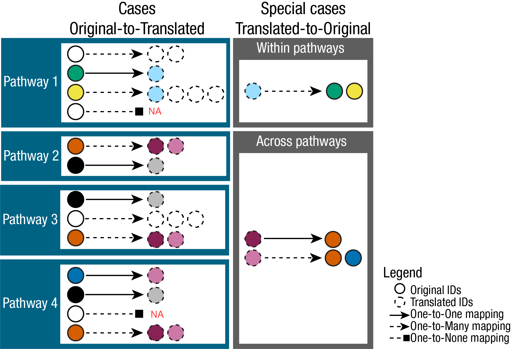
The complexities of translating metabolite IDs are demonstrated here (Fig.2). The relationships between Original IDs (e.g. KEGG) and Translated IDs (e.g. HMDB), can be quite complex and in fact we encounter one-to-one (no matches were found for the ID), one-to-none ( direct #relationship was established), one-to-many (multiple matches were found for the ID. i.e. it is ambiguously mapped) and many-to-many ( considers the relationships between the Translated IDs to Original IDs , where a translated ID ambiguously maps back to multiple different Original IDs) mappings.
For enrichment analysis the translation from KEGG IDs to HMDB IDs increases the pathways size, i.e. how many metabolites are in the pathway “Glycolysis / Gluconeogenesis - Homo sapiens (human)”, which would in turn inflate/deflate the enrichment results and hence it would be desired to keep the number of metabolites in a pathway consistent.

Fig. 2: Mapping problems in prior knowledge metabolite-sets when translating metabolite IDs.

Because of this complexity the output of MetaProViz::TranslateID() includes not only the Translation table showcased above, but additionally information about the mapping ambiguity as well as a summary of the relationships between the Original and Translated IDs.
Indeed, the translation of e.g. KEGG to hmdb and pubchem includes multiple data frames including a summary of the mapping occurrences:

names(KEGG_Pathways_Translated)
#> [1] "TranslatedDF"             "TranslatedDF_MappingInfo"
#> [3] "MappingSummary_hmdb"      "MappingSummary_pubchem"

MappingSummary_hmdb
term	many_to_many	one_to_many	one_to_none	total	to_many	to_none	to_total	from_many	from_one	from_total	one_to_one	to_one	scope
Glycolysis / Gluconeogenesis - Homo sapiens (human)	22	68	6	96	25	6	31	11	69	80	0	0	group
Citrate cycle (TCA cycle) - Homo sapiens (human)	0	48	3	51	17	3	20	0	49	49	0	0	group
Pentose phosphate pathway - Homo sapiens (human)	38	60	10	109	26	10	37	19	62	81	1	1	group
Ascorbate and aldarate metabolism - Homo sapiens (human)	18	96	26	143	28	26	57	9	100	109	3	3	group
Starch and sucrose metabolism - Homo sapiens (human)	0	78	19	98	17	19	37	0	80	80	1	1	group
Amino sugar and nucleotide sugar metabolism - Homo sapiens (human)	98	134	72	304	47	72	119	49	135	184	0	0	group

We also have the ability to extract a long version of the DF that includes a row for each mapping occurrence, which can be useful for downstream analysis. Yet, this can become very large dependent on the amount of many-to-many mappings, hence by default we do not generate this summary. Within the MetaProViz::TranslateID() you can set the parameter Summary =TRUE or in case you have a dataframe that includes both, original and translated ID, you can use the function MetaProViz::MappingAmbiguity() to generate this long summary as well as the mapping summary in general.

# Option 1:
KEGG_Pathways_TranslatedSum <- MetaProViz::TranslateID(InputData= KEGG_Pathways,
                                                    SettingsInfo = c(InputID="MetaboliteID", GroupingVariable="term"),
                                                    From = c("kegg"),
                                                    To = c("hmdb", "pubchem"),
                                                    Summary =TRUE)

# Option 2:
MappingProblems <- MetaProViz::MappingAmbiguity(InputData= KEGG_Pathways_Translated[["TranslatedDF"]]%>% dplyr::rename("KEGG"="MetaboliteID"),
                                                From = "KEGG",
                                                To = "hmdb",
                                                GroupingVariable = "term",
                                                Summary=TRUE)

Long summary of mapping problems taking into account both directions, From-to-To and To-to-From.
KEGG	hmdb	term	KEGG_to_hmdb	Count(KEGG_to_hmdb)	hmdb_to_KEGG	Count(hmdb_to_KEGG)	Mapping
C00002	HMDB0000538	Calcium signaling pathway - Homo sapiens (human)	C00002 –> HMDB0000538, HMDB00538, HMDB0257997	3	HMDB0000538 –> C00002	1	one-to-many
C00002	HMDB0000538	Diabetic cardiomyopathy - Homo sapiens (human)	C00002 –> HMDB0000538, HMDB00538, HMDB0257997	3	HMDB0000538 –> C00002	1	one-to-many
C00024	HMDB01206	Insulin resistance - Homo sapiens (human)	C00024 –> HMDB0001206, HMDB01206, HMDB0247926	3	HMDB01206 –> C00024	1	one-to-many
C00024	HMDB01206	Lysine degradation - Homo sapiens (human)	C00024 –> HMDB0001206, HMDB01206, HMDB0247926	3	HMDB01206 –> C00024	1	one-to-many

in the table it is shown that the KEGG ID C00002 maps to 3 different HMDB IDs, and it is shown that one of those HMDB IDs HMDB0000538 maps to one KEGG ID, hence this Mapping is one-to-many. The other two HMDB Ids are also in the table and it is checked to how many KEGG IDs they map. Additionally, we have passed GroupingVariable = "term" as we have pathways, which also means each of those mappings is checked within a pathway and across pathways (e.g. C00002 is shown twice, for two different terms).
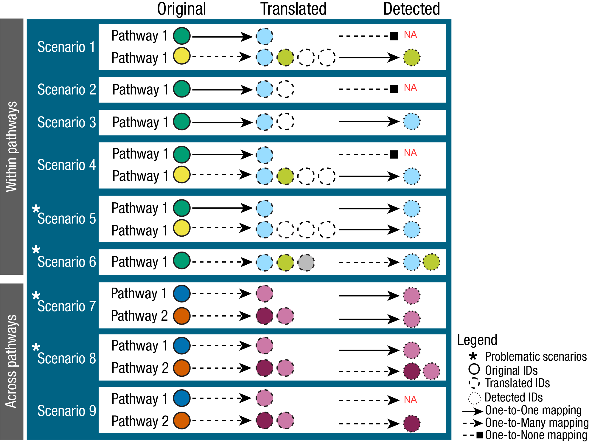
In fact, to perform enrichment analysis we need a column source (=e.g. term) and we would want to keep the metabolite IDs across pathways consistent, avoid ambiguous mapping as much as possible (many-to-many mapping), and have this metabolite ID selection guided by any IDs we might have available to us in our measured input data (Fig. 3). This is crucial to circumvent inflation or deflation of metabolite-sets, which in turn will affect the enrichment analysis results. In the next section 4., we will elaborate on this.

Fig. 3: Mapping problems in prior knowledge metabolite-sets when translating metabolite IDs and the connection to detected (measured input metabolites).

4. Metabolite IDs in measured data

4.1 Use measured Metabolite IDs to guide the selection of PK IDs

The measured metabolite IDs can be used to guide the selection of PK IDs. This is crucial to circumvent inflation or deflation of metabolite-sets, which in turn will affect the enrichment analysis results.
This is something we are currently working on and hope to provide within the next release, so stay tuned.

4.2. Assigning Metabolite IDs to measured data

The difficulty with assigning metabolite IDs to measured data is the uncertainty in the detection of metabolites. Indeed, differentiation of structural isomers (both constitutional isomers and stereoisomers) as for example the distinction between enantiomers. This leads to loss of information and hence uncertainty is assigning metabolite IDs.
One example is the metabolite Alanine, which can occur in its L- or D- form. If in an experiment those enantiomers have not been distinguished, the correct way would be to either assign two metabolite IDs (L- and D-Alanine) or a more general Alanine ID without chiral information. Yet, in reality this is not as trivial:

Available Alanine IDs in HMDB and ChEBI.
TrivialName	HMDB	ChEBI	KEGG	PubChem
D-Alanine	HMDB0001310	15570	C00133	71080
L-Alanine	HMDB0000161	16977	C00041	5950
Alanine	NA	16449	C01401	602
Alanine zwitterion	NA	66916	NA	57383916

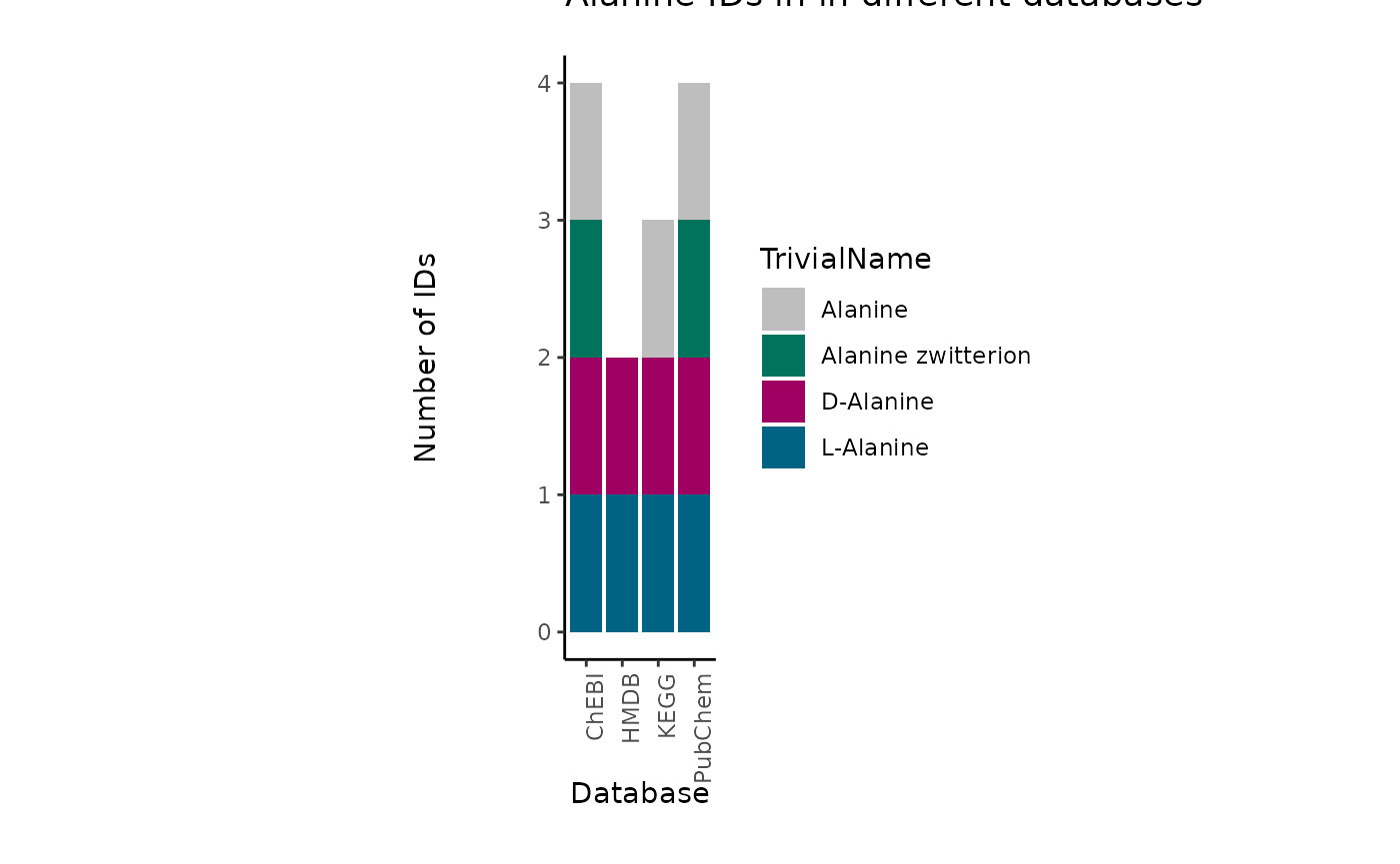
Indeed, dependent on the database, the Alanine metabolite can have different IDs available:

For instance, if we want to assign a HMDB ID, we have to assign both “HMDB0001310”, “HMDB0000161” to the metabolite Alanine, for ChEBI we could assign only one, “16449”, but this may lead to other problems as the ChEBI ID is not specific and may not be part of certain metabolic pathways. The reason for this is that substrate chirality is critical to enzymatic processes and stereo selectivity of enzymes to be homochiral with predominance of one particular enantiomer (e.g. D-sugars, L-amino acids, etc.).
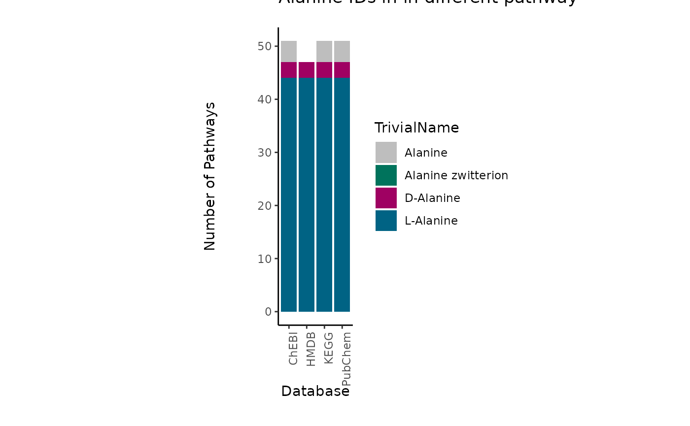
To showcase the severity of this problem, we can look at the occurrence of those metabolites in metabolic pathways across different databases. To do so we searched for those metabolite IDs in the RaMP database (Braisted et al. 2023) and extracted the pathways they are part of:

Alanine IDs in HMDB and ChEBI mapped to pathways from wiki, KEGG and Reactome using RamP.
TrivialName	ID	Database	PathwayCount
L-Alanine	16977	ChEBI	44
L-Alanine	5950	PubChem	44
L-Alanine	C00041	KEGG	44
L-Alanine	HMDB0000161	HMDB	44
D-Alanine	15570	ChEBI	3
D-Alanine	71080	PubChem	3
D-Alanine	C00133	KEGG	3
D-Alanine	HMDB0001310	HMDB	3
Alanine zwitterion	57383916	PubChem	0
Alanine zwitterion	66916	ChEBI	0
Alanine	16449	ChEBI	4
Alanine	602	PubChem	4
Alanine	C01401	KEGG	4

This showcases if we choose the ChEBI ID for Alanine (ChEBI ID 16449), if experimentally the distinction was not possible, we will not map to any pathway even though the metabolite is part of many pathways. Hence, we recommend to assign multiple IDs to a measured ID, where specificity in detection is not given.

5. Run enrichment analysis

There are two options:
1. Over Representation Analysis (ORA) that determines if a set of features (=metabolic pathways) are over-represented in the selection of features (=metabolites) from the data in comparison to all measured features (metabolites) using the Fishers exact test MetaProViz::ClusterORA. This can be applied to clusters of metabolites as for example the results from MetaProViz::MCA_2Cond() or MetaProViz::CoRe() function. If you want to have more details on these clustering methods please visit the vignette Standard Metabolomics or CoRe Metabolomics.

2. Enrichment analysis on standard differential analysis results. We offer ORA MetaProViz::StandardORA, but there are many other statistical tests that can be used for enrichment analysis. The full scope of different methods is beyond the scope of MetaProViz, but are available in decoupleR (Badia-I-Mompel et al. 2022) packages from our group.

Session information

#> R version 4.4.2 (2024-10-31)
#> Platform: x86_64-pc-linux-gnu
#> Running under: Ubuntu 24.04.1 LTS
#> 
#> Matrix products: default
#> BLAS:   /usr/lib/x86_64-linux-gnu/openblas-pthread/libblas.so.3 
#> LAPACK: /usr/lib/x86_64-linux-gnu/openblas-pthread/libopenblasp-r0.3.26.so;  LAPACK version 3.12.0
#> 
#> locale:
#>  [1] LC_CTYPE=C.UTF-8       LC_NUMERIC=C           LC_TIME=C.UTF-8        LC_COLLATE=C.UTF-8     LC_MONETARY=C.UTF-8   
#>  [6] LC_MESSAGES=C.UTF-8    LC_PAPER=C.UTF-8       LC_NAME=C              LC_ADDRESS=C           LC_TELEPHONE=C        
#> [11] LC_MEASUREMENT=C.UTF-8 LC_IDENTIFICATION=C   
#> 
#> time zone: UTC
#> tzcode source: system (glibc)
#> 
#> attached base packages:
#> [1] stats     graphics  grDevices utils     datasets  methods   base     
#> 
#> other attached packages:
#>  [1] lubridate_1.9.4  forcats_1.0.0    stringr_1.5.1    purrr_1.0.2      readr_2.1.5      tibble_3.2.1    
#>  [7] tidyverse_2.0.0  tidyr_1.3.1      dplyr_1.1.4      magrittr_2.0.3   MetaProViz_2.1.3 ggplot2_3.5.1   
#> 
#> loaded via a namespace (and not attached):
#>   [1] DBI_1.2.3         gridExtra_2.3     logger_0.4.0      readxl_1.4.3      rlang_1.1.4       compiler_4.4.2   
#>   [7] RSQLite_2.3.9     systemfonts_1.1.0 vctrs_0.6.5       reshape2_1.4.4    rvest_1.0.4       pkgconfig_2.0.3  
#>  [13] crayon_1.5.3      fastmap_1.2.0     backports_1.5.0   labeling_0.4.3    rmarkdown_2.29    tzdb_0.4.0       
#>  [19] ggbeeswarm_0.7.2  ragg_1.3.3        bit_4.5.0.1       xfun_0.49         cachem_1.1.0      jsonlite_1.8.9   
#>  [25] progress_1.2.3    blob_1.2.4        later_1.4.1       broom_1.0.7       parallel_4.4.2    prettyunits_1.2.0
#>  [31] R6_2.5.1          bslib_0.8.0       stringi_1.8.4     limma_3.58.1      car_3.1-3         jquerylib_0.1.4  
#>  [37] cellranger_1.1.0  Rcpp_1.0.13-1     knitr_1.49        R.utils_2.12.3    igraph_2.1.2      timechange_0.3.0 
#>  [43] tidyselect_1.2.1  rstudioapi_0.17.1 abind_1.4-8       yaml_2.3.10       curl_6.0.1        plyr_1.8.9       
#>  [49] withr_3.0.2       inflection_1.3.6  evaluate_1.0.1    desc_1.4.3        zip_2.3.1         xml2_1.3.6       
#>  [55] pillar_1.10.0     ggpubr_0.6.0      carData_3.0-5     checkmate_2.3.2   generics_0.1.3    vroom_1.6.5      
#>  [61] hms_1.1.3         munsell_0.5.1     scales_1.3.0      gtools_3.9.5      OmnipathR_3.15.2  glue_1.8.0       
#>  [67] tools_4.4.2       ggsignif_0.6.4    fs_1.6.5          XML_3.99-0.17     grid_4.4.2        qcc_2.7          
#>  [73] colorspace_2.1-1  patchwork_1.3.0   beeswarm_0.4.0    vipor_0.4.7       Formula_1.2-5     cli_3.6.3        
#>  [79] rappdirs_0.3.3    kableExtra_1.4.0  textshaping_0.4.1 viridisLite_0.4.2 svglite_2.1.3     gtable_0.3.6     
#>  [85] R.methodsS3_1.8.2 rstatix_0.7.2     hash_2.2.6.3      selectr_0.4-2     sass_0.4.9        digest_0.6.37    
#>  [91] ggrepel_0.9.6     htmlwidgets_1.6.4 farver_2.1.2      memoise_2.0.1     htmltools_0.5.8.1 pkgdown_2.1.1    
#>  [97] R.oo_1.27.0       factoextra_1.0.7  lifecycle_1.0.4   httr_1.4.7        statmod_1.5.0     bit64_4.5.2      
#> [103] MASS_7.3-61

Bibliography

Badia-I-Mompel, Pau, Jesús Vélez Santiago, Jana Braunger, Celina Geiss, Daniel Dimitrov, Sophia Müller-Dott, Petr Taus, et al. 2022. “decoupleR: Ensemble of Computational Methods to Infer Biological Activities from Omics Data.” Bioinformatics Advances 2 (1): vbac016. https://doi.org/10.1093/bioadv/vbac016.

Braisted, John, Andrew Patt, Cole Tindall, Timothy Sheils, Jorge Neyra, Kyle Spencer, Tara Eicher, and Ewy A Mathé. 2023. “RaMP-DB 2.0: A Renovated Knowledgebase for Deriving Biological and Chemical Insight from Metabolites, Proteins, and Genes.” Bioinformatics, no. 1 (January). https://doi.org/10.1093/bioinformatics/btac726.

Castanza, Anthony Scott, Jill Marie Recla, David Eby, Helga Thorvaldsdottir, Carol J. Bult, and Jill P Mesirov. 2022. “The Molecular Signatures Database Revisited: Extending Support for Mouse Data.” BioRxiv, October. https://doi.org/10.1101/2022.10.24.513539.

Dugourd, Aurelien, Christoph Kuppe, Marco Sciacovelli, Enio Gjerga, Attila Gabor, Kristina B Emdal, Vitor Vieira, et al. 2021. “Causal Integration of Multi-Omics Data with Prior Knowledge to Generate Mechanistic Hypotheses.” Molecular Systems Biology, no. 1 (January): e9730. https://doi.org/10.15252/msb.20209730.

Farr, Elias, Daniel Dimitrov, Christina Schmidt, Denes Turei, Sebastian Lobentanzer, Aurelien Dugourd, and Julio Saez-Rodriguez. 2024. “MetalinksDB: A Flexible and Contextualizable Resource of Metabolite-Protein Interactions.” Briefings in Bioinformatics, no. 4 (May). https://doi.org/10.1093/bib/bbae347.

Kanehisa, M, and S Goto. 2000. “KEGG: Kyoto Encyclopedia of Genes and Genomes.” Nucleic Acids Research 28 (1): 27–30. https://doi.org/10.1093/nar/28.1.27.

Sciacovelli, Marco, Aurelien Dugourd, Lorea Valcarcel Jimenez, Ming Yang, Efterpi Nikitopoulou, Ana S H Costa, Laura Tronci, et al. 2022. “Dynamic Partitioning of Branched-Chain Amino Acids-Derived Nitrogen Supports Renal Cancer Progression.” Nature Communications 13 (1): 7830. https://doi.org/10.1038/s41467-022-35036-4.

Christina Schmidt

Macabe Daley