MetSigDB

In this tutorial we take a closer look at the prior knowledge resources collected in MetSigDB:
- 1. to retrieve all MetSigDB resources and bring them into one common format.

- 2. to compare the resources by size, specificity and redundancy.

- 3. to cluster the terms within each resource and understand its internal structure.

- 4. to choose a resource that fits your data and research question.

MetSigDB (Metabolite signature database) is the collection of metabolite sets accessible via the metsigdb_*() functions of MetaProViz. How to load single resources, link them to your measured data and translate metabolite IDs is shown in the vignette Prior Knowledge - Access & Integration, which we recommend to read first. Here, we focus on the resources themselves: before using a resource for enrichment analysis, it is worth knowing how large its terms are, how often the same metabolite appears in different terms, and which terms are (nearly) redundant, since all of this shapes the enrichment results.

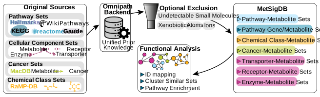
Fig. 1 summarises how MetSigDB is built and used. The original sources are accessed via OmniPath and RaMP-DB in the backend and turned into unified sets of pathway-, chemical class-, cancer- and protein-metabolite sets. Metabolites that carry little biological information (ions, undetectable small molecules, atoms and xenobiotics) can optionally be excluded. The resulting prior knowledge is then used for ID mapping, clustering of similar sets and pathway enrichment.

Fig. 1: Overview of MetSigDB: original sources, unified metabolite set types, optional metabolite exclusion and downstream functional analysis.

Important Information: All resources are retrieved live at the time this vignette is built. Since the upstream resources are updated over time, the exact numbers in the tables and plots below can change between versions of this vignette.

Terminology

Every MetSigDB resource can be described as a set of terms and their targets:

• A term is the set name: a pathway (KEGG, Reactome, WikiPathways, Gaude, Hallmarks), a chemical class (ClassyFire), a protein (MetaLinks) or a cancer association (MACdb).
• A target is a member of the set: a metabolite, or, for the gene-metabolite sets of Gaude and Hallmarks, also a metabolic enzyme.
• An interaction is a unique term-target pair.

From these, we derive two properties that we use throughout this tutorial:

• Term size is the number of targets per term. Broad terms have many targets and high coverage, but are less specific.
• Recurrence is the number of terms that contain a target. Highly recurrent targets (e.g. ATP or NADH) link many terms with each other and can produce overlapping enrichment results.

The benchmark includes KEGG (Kanehisa et al. 2017), Reactome (Milacic et al. 2024), WikiPathways (Agrawal et al. 2024), ClassyFire (Djoumbou Feunang et al. 2016), MetaLinks (Farr et al. 2024), MACdb (Sun et al. 2023), Gaude (Gaude and Frezza 2018), and Hallmarks (Liberzon et al. 2015).

First if you have not done yet, install the required dependencies and load the libraries:

# 1. Install MetaProViz from Bioconductor devel:
# if (!requireNamespace("BiocManager", quietly = TRUE)) install.packages("BiocManager")
# BiocManager::install(version = "devel")
# BiocManager::install("MetaProViz")

suppressPackageStartupMessages({
    library(MetaProViz)
    library(dplyr)
    library(tidyr)
    library(purrr)
    library(tibble)
    library(ggplot2)
    library(knitr)
    library(scales)
})

# Helper to show long tables in a scrollable box:
scrollable_table <- function(x, ...) {
    kableExtra::scroll_box(knitr::kable(x, format = "html", ...), height = "400px", width = "100%")
}

Retrieve and harmonise the resources

Harmonise the metabolite IDs

Each resource uses its own metabolite ID type, and even the same ID type is not always written the same way (e.g. “HMDB0000161” versus “HMDB00161”, or “16977” versus “CHEBI:16977”). To count unique targets correctly, we first define small helpers that bring every ID into one canonical form.

normalise_id <- function(x, prefix, width = 0L) {
    x <- trimws(as.character(x))
    digits <- gsub("[^0-9]", "", x)
    digits[is.na(x) | x == "" | digits == ""] <- NA_character_
    if (width > 0L) {
        digits <- ifelse(
            is.na(digits),
            NA_character_,
            sprintf(paste0("%0", width, "d"), as.integer(digits))
        )
    }
    paste0(prefix, digits)
}

normalise_hmdb <- function(x) normalise_id(x, "HMDB", 7L)    # HMDB0000161
normalise_kegg <- function(x) normalise_id(x, "C", 5L)       # C00041
normalise_chebi <- function(x) normalise_id(x, "CHEBI:")     # CHEBI:16977
normalise_pubchem <- function(x) normalise_id(x, "CID")      # CID5950

Load all resources

Next, we load every resource with its metsigdb_*() function. The table below summarises what each resource contains and which ID type it uses:

Resource	Function	Term	Target (ID type)
KEGG	metsigdb_kegg()	Pathway	Metabolite (KEGG)
Reactome	metsigdb_reactome()	Pathway	Metabolite (ChEBI)
WikiPathways	metsigdb_wikipathways()	Pathway	Metabolite (mixed, harmonised to HMDB)
MACdb	metsigdb_macdb()	Cancer association	Metabolite (PubChem)
ClassyFire	metsigdb_chemicalclass()	Chemical class	Metabolite
MetaLinks	metsigdb_metalinks()	Protein (receptor, enzyme, transporter)	Metabolite (HMDB)
Gaude	data(gaude_pathways) + make_gene_metab_set()	Pathway	Metabolite (HMDB) and metabolic enzyme
Hallmarks	data(hallmarks) + make_gene_metab_set()	Pathway	Metabolite (HMDB) and metabolic enzyme

All metsigdb_*() functions and make_gene_metab_set() have the parameter exclude_metabolites, which removes metabolites that are part of many reactions but carry little biological information. By default (exclude_metabolites = "all") the classes “ions”, “small_molecules” (e.g. water, CO2), “xenobiotics” and “atoms” are removed; with exclude_metabolites = NULL nothing is removed. The exclusion should match the metabolite universe you use for enrichment, and we will quantify its effect in section 2.4.

Gaude and Hallmarks are gene-sets. make_gene_metab_set() adds the metabolites of the reactions catalysed by the enzymes in each gene-set, so these resources contain both metabolites and genes as targets. We wrap their creation in a small helper and label each target as metabolite or enzyme:

fetch_derived <- function(dataset, name, exclusion) {
    data(list = dataset, package = "MetaProViz", envir = environment())
    make_gene_metab_set(
        get(dataset, envir = environment()),
        metadata_info = c(Target = "gene"),
        pk_name = name,
        save_table = NULL,
        exclude_metabolites = exclusion
    )$GeneMetabSet |>
        mutate(interaction_type = if_else(
            grepl("^HMDB", feature),
            "pathway-metabolite",
            "pathway-metabolic_enzyme"
        ))
}

Now we can load all resources in one go. MetaLinks is split by its interaction_family column into receptor-, enzyme- and transporter-metabolite interactions, as these answer different biological questions.

live_resources <- function(exclusion = "all") {
    metalinks <- metsigdb_metalinks(exclude_metabolites = exclusion) |>
        collect() |>
        mutate(hmdb = normalise_hmdb(hmdb))

    list(
        kegg = metsigdb_kegg(exclude_metabolites = exclusion) |>
            mutate(MetaboliteID = normalise_kegg(MetaboliteID)),
        reactome = metsigdb_reactome(species = "Homo sapiens", exclude_metabolites = exclusion) |>
            mutate(chebi_id = normalise_chebi(chebi_id)),
        wikipathways = metsigdb_wikipathways(species = "Homo sapiens", exclude_metabolites = exclusion),
        macdb = metsigdb_macdb(exclude_metabolites = exclusion) |>
            mutate(Metabolite_PubchemID = normalise_pubchem(Metabolite_PubchemID)),
        chemicalclass = metsigdb_chemicalclass(exclude_metabolites = exclusion),
        receptor = filter(metalinks, interaction_family == "Receptor-metabolite"),
        enzyme = filter(metalinks, interaction_family == "Enzyme-metabolite"),
        transporter = filter(metalinks, interaction_family == "Transporter-metabolite"),
        gaude = fetch_derived("gaude_pathways", "gaude_pathways", exclusion),
        hallmarks = fetch_derived("hallmarks", "hallmarks", exclusion)
    )
}

Harmonise WikiPathways

WikiPathways is curated by a community and contains a mix of identifier types (HMDB, ChEBI and PubChem) within the same column. To make it comparable to the other resources, we keep the HMDB IDs as they are and translate ChEBI and PubChem IDs to HMDB via RaMP-DB using OmnipathR::translate_ids(). Metabolites that cannot be translated keep hmdb = NA.

harmonise_wikipathways <- function(wp) {
    wp <- wp |>
        mutate(
            .row = row_number(),
            raw = trimws(as.character(metabolite_id)),
            hmdb = if_else(grepl("^HMDB[0-9]+$", raw, ignore.case = TRUE), normalise_hmdb(raw), NA_character_),
            chebi = if_else(grepl("^CHEBI[:_][0-9]+$", raw, ignore.case = TRUE), gsub("[^0-9]", "", raw), NA_character_),
            pubchem = if_else(grepl("^(CID|PUBCHEM[:_])[0-9]+$", raw, ignore.case = TRUE), gsub("[^0-9]", "", raw), NA_character_)
        )

    translate <- function(column, type, output) {
        x <- wp |> filter(!is.na(.data[[column]])) |> select(.row, value = all_of(column))
        if (!nrow(x)) return(tibble(.row = integer(), !!output := character()))
        OmnipathR::translate_ids(
            x, value = type, !!output := "hmdb", ramp = TRUE,
            entity_type = "smol", keep_untranslated = TRUE, return_df = TRUE
        ) |>
            select(.row, all_of(output))
    }

    wp |>
        left_join(translate("chebi", "chebi", "hmdb_chebi"), by = ".row") |>
        left_join(translate("pubchem", "pubchem", "hmdb_pubchem"), by = ".row") |>
        mutate(hmdb = coalesce(hmdb, normalise_hmdb(hmdb_chebi), normalise_hmdb(hmdb_pubchem))) |>
        select(-.row, -raw, -chebi, -pubchem, -hmdb_chebi, -hmdb_pubchem)
}

Combine everything into one table

Finally, we bring all resources into one long table with the columns resource, group, type, term and target. Each row is one interaction. Gaude and Hallmarks are split into their metabolite-pathway and metabolite-enzyme parts, since metabolites and genes have very different set sizes.

as_edges <- function(x) {
    bind_rows(
        transmute(x$kegg, resource = "KEGG", group = "Pathway", type = "pathway-metabolite",
            term = term, target = MetaboliteID),
        transmute(x$reactome, resource = "Reactome", group = "Pathway", type = "pathway-metabolite",
            term = pathway_name, target = chebi_id),
        transmute(x$wikipathways, resource = "WikiPathways", group = "Pathway", type = "pathway-metabolite",
            term = pathway_name, target = hmdb),
        transmute(x$macdb, resource = "MACdb", group = "Cancer association", type = "metabolite-cancer",
            term = term, target = Metabolite_PubchemID),
        transmute(x$chemicalclass, resource = "ClassyFire", group = "Annotation", type = "metabolite-annotation",
            term = ClassyFire_class, target = class_source_id),
        imap_dfr(x[c("receptor", "enzyme", "transporter")], ~ transmute(.x,
            resource = paste("MetaLinks", .y), group = "Interaction", type = "metabolite-protein",
            term = gene_symbol, target = hmdb)),
        imap_dfr(x[c("gaude", "hallmarks")], ~ transmute(.x,
            resource = .y, group = "Derived pathway", type = interaction_type,
            term = term, target = feature))
    ) |>
        mutate(resource = case_when(
            resource == "gaude" & type == "pathway-metabolite" ~ "Gaude: metabolite-pathway",
            resource == "gaude" & type == "pathway-metabolic_enzyme" ~ "Gaude: metabolite-enzyme",
            resource == "hallmarks" & type == "pathway-metabolite" ~ "Hallmarks: metabolite-pathway",
            resource == "hallmarks" & type == "pathway-metabolic_enzyme" ~ "Hallmarks: metabolite-enzyme",
            TRUE ~ resource
        )) |>
        filter(!is.na(term), term != "", !is.na(target), target != "") |>
        distinct()
}

We retrieve all resources twice: once with the default exclusion ("all") and once without any exclusion (NULL), so we can quantify the effect of the exclusion later on.

default_raw <- live_resources("all")
default_raw$wikipathways <- harmonise_wikipathways(default_raw$wikipathways)

none_raw <- live_resources(NULL)
none_raw$wikipathways <- harmonise_wikipathways(none_raw$wikipathways)

edges <- as_edges(default_raw)
edges_none <- as_edges(none_raw)

Preview of the combined table edges: one example interaction per resource.

resource	group	type	term	target
ClassyFire	Annotation	metabolite-annotation	Carboxylic acids and derivatives	HMDB0000001
Gaude: metabolite-enzyme	Derived pathway	pathway-metabolic_enzyme	Sphingolipid Metabolism	A4GALT
Gaude: metabolite-pathway	Derived pathway	pathway-metabolite	Sphingolipid Metabolism	HMDB0000302
Hallmarks: metabolite-enzyme	Derived pathway	pathway-metabolic_enzyme	HALLMARK_ADIPOGENESIS	FABP4
Hallmarks: metabolite-pathway	Derived pathway	pathway-metabolite	HALLMARK_FATTY_ACID_METABOLISM	HMDB0000225
KEGG	Pathway	pathway-metabolite	Glycolysis / Gluconeogenesis	C00022
MACdb	Cancer association	metabolite-cancer	ADC, SCC, NSCLC	CID102172
MetaLinks enzyme	Interaction	metabolite-protein	UBA6	HMDB0000045
MetaLinks receptor	Interaction	metabolite-protein	HTR3E	HMDB0000073
MetaLinks transporter	Interaction	metabolite-protein	SLC5A10	HMDB0000660
Reactome	Pathway	pathway-metabolite	Interleukin-6 signaling	CHEBI:30616
WikiPathways	Pathway	pathway-metabolite	Glutathione metabolism	HMDBNA

Resource composition

With all resources in one table, we can describe each of them with the same set of numbers. The function below computes three summaries per resource: the footprint (how many terms, targets and interactions), the term size distribution and the target recurrence.

composition <- function(edges) {
    footprint <- edges |>
        group_by(resource, group, type) |>
        summarise(
            terms = n_distinct(term),
            targets = n_distinct(target),
            interactions = n(),
            mean_targets_per_term = interactions / terms,
            mean_terms_per_target = interactions / targets,
            .groups = "drop"
        )

    term_size <- edges |>
        count(resource, group, type, term, name = "targets_per_term") |>
        group_by(resource, group, type) |>
        summarise(
            min_targets = min(targets_per_term),
            median_targets = median(targets_per_term),
            mean_targets = mean(targets_per_term),
            max_targets = max(targets_per_term),
            .groups = "drop"
        )

    recurrence <- edges |>
        count(resource, group, type, target, name = "terms_per_target") |>
        mutate(bucket = cut(terms_per_target, c(0, 1, 2, 5, Inf), labels = c("1", "2", "3-5", "6+"))) |>
        count(resource, group, type, bucket, name = "targets") |>
        group_by(resource, group, type) |>
        mutate(share = targets / sum(targets)) |>
        ungroup()

    list(footprint = footprint, term_size = term_size, recurrence = recurrence)
}

bench <- composition(edges)
bench_none <- composition(edges_none)

Footprint

The footprint tells us how much of the metabolite (and gene) space a resource covers. A resource with many targets is more likely to cover your measured metabolites, whilst the number of terms determines how many tests an enrichment analysis performs.

scrollable_table(bench$footprint, digits = 2, caption = "Resource footprint (default exclusion)")

Resource footprint (default exclusion)

resource	group	type	terms	targets	interactions	mean_targets_per_term	mean_terms_per_target
ClassyFire	Annotation	metabolite-annotation	409	145716	145716	356.27	1.00
Gaude: metabolite-enzyme	Derived pathway	pathway-metabolic_enzyme	96	1453	1932	20.12	1.33
Gaude: metabolite-pathway	Derived pathway	pathway-metabolite	90	822	3822	42.47	4.65
Hallmarks: metabolite-enzyme	Derived pathway	pathway-metabolic_enzyme	50	4384	7322	146.44	1.67
Hallmarks: metabolite-pathway	Derived pathway	pathway-metabolite	48	753	4536	94.50	6.02
KEGG	Pathway	pathway-metabolite	453	6645	19055	42.06	2.87
MACdb	Cancer association	metabolite-cancer	212	5404	17939	84.62	3.32
MetaLinks enzyme	Interaction	metabolite-protein	2516	911	11936	4.74	13.10
MetaLinks receptor	Interaction	metabolite-protein	671	373	9558	14.24	25.62
MetaLinks transporter	Interaction	metabolite-protein	481	385	3067	6.38	7.97
Reactome	Pathway	pathway-metabolite	2448	3197	35741	14.60	11.18
WikiPathways	Pathway	pathway-metabolite	693	1920	6638	9.58	3.46

footprint_long <- pivot_longer(bench$footprint, c(terms, targets, interactions), names_to = "metric", values_to = "count")
ggplot(footprint_long, aes(resource, count, fill = metric)) +
    geom_col(position = "dodge") +
    coord_flip() +
    labs(title = "Resource footprint", x = NULL, y = "Count") +
    theme_minimal()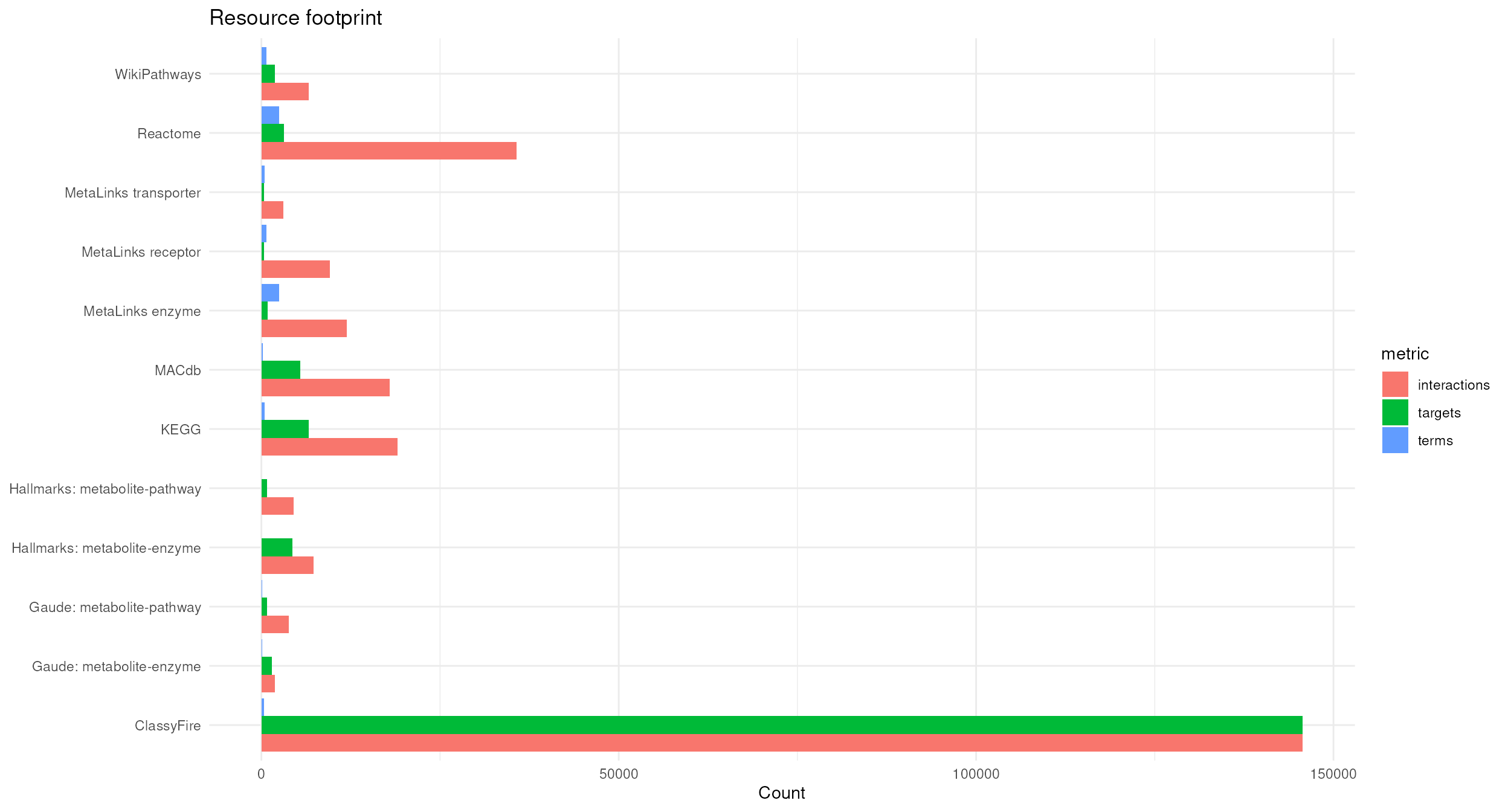

When reading the footprint, compare mean_targets_per_term and mean_terms_per_target: the first is a rough measure of how broad the terms are, the second of how much the terms share their targets.

Term size

The mean term size can be dominated by a few very large terms, hence we look at the full distribution and plot the median.

scrollable_table(bench$term_size, digits = 2, caption = "Term-size distribution")

Term-size distribution

resource	group	type	min_targets	median_targets	mean_targets	max_targets
ClassyFire	Annotation	metabolite-annotation	1	10.0	356.27	62599
Gaude: metabolite-enzyme	Derived pathway	pathway-metabolic_enzyme	1	15.5	20.12	82
Gaude: metabolite-pathway	Derived pathway	pathway-metabolite	1	21.5	42.47	199
Hallmarks: metabolite-enzyme	Derived pathway	pathway-metabolic_enzyme	32	180.0	146.44	200
Hallmarks: metabolite-pathway	Derived pathway	pathway-metabolite	1	56.0	94.50	362
KEGG	Pathway	pathway-metabolite	1	11.0	42.06	3234
MACdb	Cancer association	metabolite-cancer	1	25.0	84.62	1659
MetaLinks enzyme	Interaction	metabolite-protein	1	2.0	4.74	89
MetaLinks receptor	Interaction	metabolite-protein	1	4.0	14.24	65
MetaLinks transporter	Interaction	metabolite-protein	1	3.0	6.38	90
Reactome	Pathway	pathway-metabolite	1	5.0	14.60	1645
WikiPathways	Pathway	pathway-metabolite	1	5.0	9.58	468

ggplot(bench$term_size, aes(reorder(resource, median_targets), median_targets, fill = type)) +
    geom_col() +
    coord_flip() +
    labs(title = "Median targets per term", x = NULL, y = "Median") +
    theme_minimal()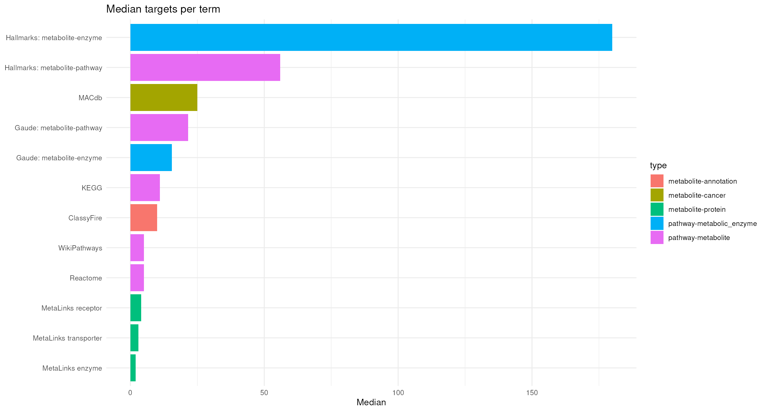

Resources with small median term sizes (e.g. single proteins in MetaLinks) give very specific, but sparse results: with only a handful of targets per term, few of them may be measured in your data. Resources with large terms (e.g. broad chemical classes or large pathways) will nearly always overlap with your data, but an enriched term is then less informative. Many enrichment methods also filter terms by size, so check which terms of a resource survive your size cut-offs.

Target recurrence

Recurrence shows which share of targets is unique to one term (“1”) and which share is found in many terms (“6+”).

ggplot(bench$recurrence, aes(resource, share, fill = bucket)) +
    geom_col() +
    coord_flip() +
    scale_y_continuous(labels = percent) +
    labs(title = "Target recurrence", x = NULL, y = "Share of targets", fill = "Terms per target") +
    theme_minimal()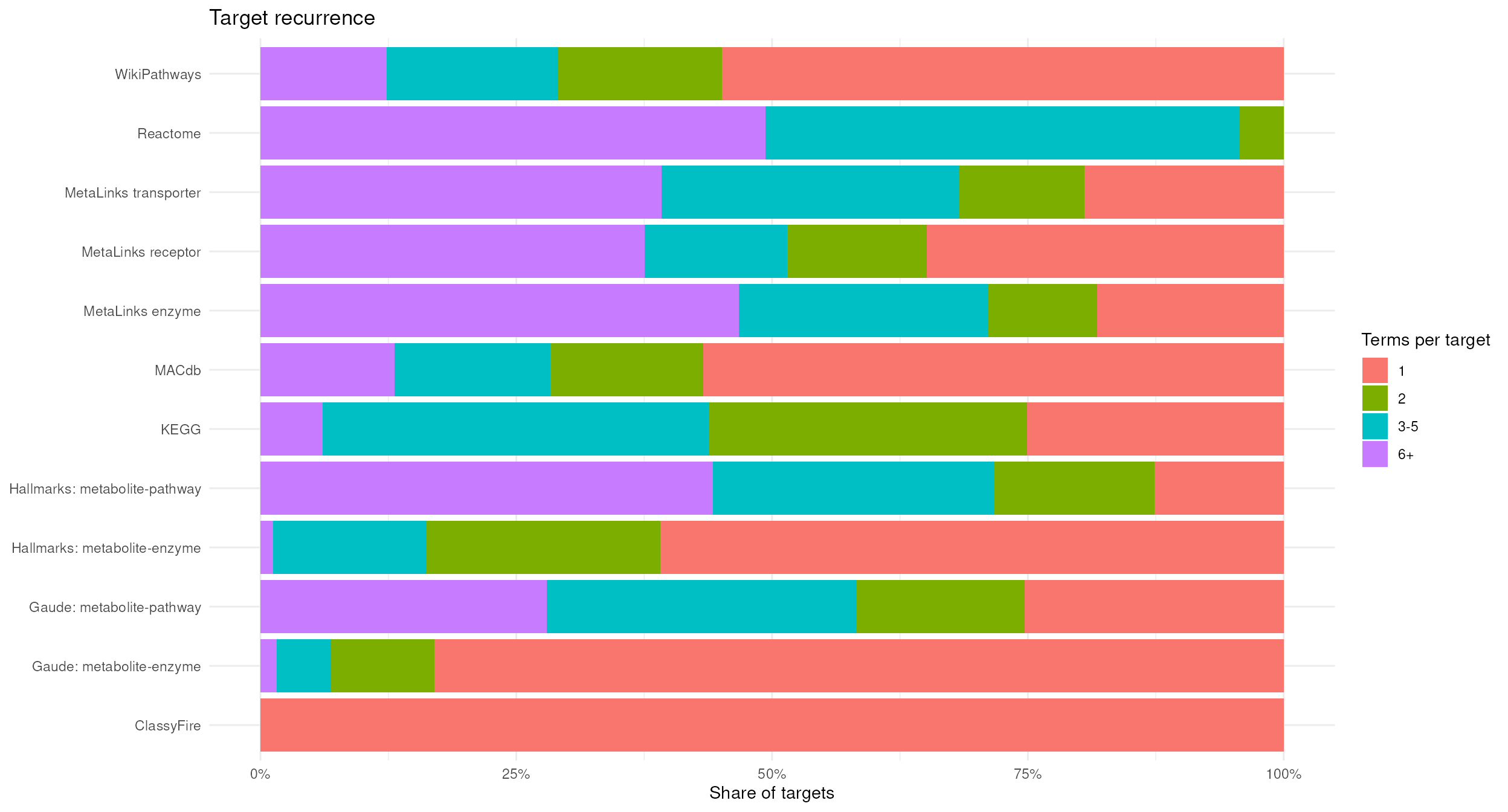

ClassyFire assigns every metabolite to its chemical classes, so recurrence there reflects the class hierarchy rather than biological redundancy. In pathway resources, a high share of recurrent targets means that a single changed metabolite can make several terms appear enriched at the same time. These are exactly the resources in which clustering the terms (section 3) helps to group redundant results.

Effect of excluding metabolites

Finally, we compare the default exclusion ("all") with no exclusion (NULL). For each resource we compute the change in targets and interactions:

exclusion <- full_join(
    bench_none$footprint, bench$footprint,
    by = c("resource", "group", "type"),
    suffix = c("_none", "_default")
) |>
    mutate(
        across(where(is.numeric), ~ replace_na(.x, 0)),
        delta_targets = targets_default - targets_none,
        delta_interactions = interactions_default - interactions_none,
        pct_delta_targets = if_else(targets_none > 0, delta_targets / targets_none, NA_real_),
        pct_delta_interactions = if_else(interactions_none > 0, delta_interactions / interactions_none, NA_real_)
    )

scrollable_table(
    select(exclusion, resource, type, targets_none, targets_default, delta_targets, pct_delta_targets,
        interactions_none, interactions_default, delta_interactions, pct_delta_interactions),
    digits = 3, caption = "Effect of the default exclusion"
)

Effect of the default exclusion

resource	type	targets_none	targets_default	delta_targets	pct_delta_targets	interactions_none	interactions_default	delta_interactions	pct_delta_interactions
ClassyFire	metabolite-annotation	145741	145716	-25	0.000	145741	145716	-25	0.000
Gaude: metabolite-enzyme	pathway-metabolic_enzyme	1453	1453	0	0.000	1932	1932	0	0.000
Gaude: metabolite-pathway	pathway-metabolite	830	822	-8	-0.010	3899	3822	-77	-0.020
Hallmarks: metabolite-enzyme	pathway-metabolic_enzyme	4384	4384	0	0.000	7322	7322	0	0.000
Hallmarks: metabolite-pathway	pathway-metabolite	761	753	-8	-0.011	4613	4536	-77	-0.017
KEGG	pathway-metabolite	6671	6645	-26	-0.004	19586	19055	-531	-0.027
MACdb	metabolite-cancer	5407	5404	-3	-0.001	17953	17939	-14	-0.001
MetaLinks enzyme	metabolite-protein	921	911	-10	-0.011	14045	11936	-2109	-0.150
MetaLinks receptor	metabolite-protein	380	373	-7	-0.018	9827	9558	-269	-0.027
MetaLinks transporter	metabolite-protein	394	385	-9	-0.023	3526	3067	-459	-0.130
Reactome	pathway-metabolite	3223	3197	-26	-0.008	38177	35741	-2436	-0.064
WikiPathways	pathway-metabolite	1920	1920	0	0.000	6638	6638	0	0.000

ggplot(exclusion, aes(resource, pct_delta_targets, fill = type)) +
    geom_col() +
    coord_flip() +
    scale_y_continuous(labels = percent) +
    labs(title = "Target change after default exclusion", x = NULL, y = "Change") +
    theme_minimal()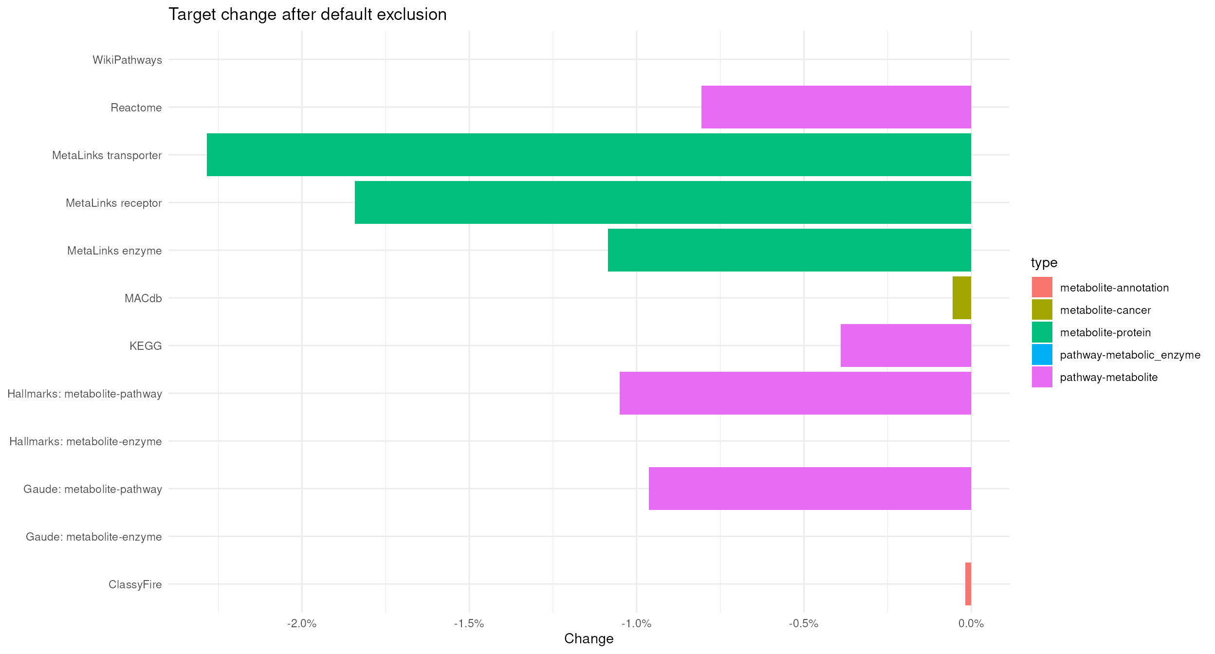

ggplot(exclusion, aes(resource, pct_delta_interactions, fill = type)) +
    geom_col() +
    coord_flip() +
    scale_y_continuous(labels = percent) +
    labs(title = "Interaction change after default exclusion", x = NULL, y = "Change") +
    theme_minimal()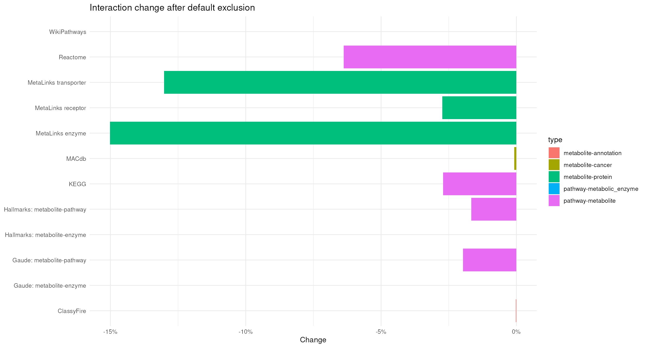

The excluded metabolites are few, but they are typically very recurrent (e.g. water or protons are part of almost every pathway). Hence, a small change in targets can come with a much larger change in interactions. Resources without a metabolite-level change, such as the enzyme parts of Gaude and Hallmarks, serve as a reference.

Clustering complete resources

The composition summaries describe each resource as a whole. To see which terms are redundant, we cluster the terms of each resource based on their shared targets using cluster_pk().

How cluster_pk() works

cluster_pk() computes a similarity between all pairs of terms, removes weak similarities, assigns the terms to clusters and draws the result as a graph with viz_graph(). In the graph each node is a term, each edge connects two terms with shared targets, and the coloured background marks a cluster. The most important parameters are:

Parameter	What it does
similarity	How similar two terms are. "jaccard" = shared targets / all targets of both terms; strict for terms of very different size. "overlap_coefficient" = shared targets / targets of the smaller term; permissive, so a small term nested in a large one gets a similarity of 1.
threshold	Similarities below this value are ignored when building the clusters. A high threshold yields few, tight clusters; a low threshold yields large, loose clusters.
clust	Clustering method. "community" uses Louvain community detection on the weighted graph, "components" uses connected components, "hierarchical" uses hierarchical clustering.
min	Minimum cluster size; terms in smaller clusters are labelled “None”.
plot_threshold	Similarities below this value are not drawn as edges. This only affects the plot, not the clusters.
min_degree	Terms with fewer edges than this are not drawn. This only affects the plot, not the clusters.
node_size_column	Column used to scale the nodes; here the number of targets per term.

The clustering and the plot are therefore controlled separately: threshold and min decide the clusters, whilst plot_threshold and min_degree decide what is shown.

Important Information: There is no correct threshold. The values used below are arbitrary and were chosen per resource to show a mix of clustering strengths, from strict (few, tight clusters) to loose (large clusters with weaker connections). The similarity metric, thresholds, degree filter and layout can change the graph substantially, so treat them as starting points and vary them for your own question. A seed is set before each call to make the community detection and the graph layout reproducible.

ClassyFire is not clustered: it is a hierarchical annotation, in which overlap between classes reflects the class hierarchy rather than redundancy.

Prepare the inputs

cluster_pk() takes a long table with one term-target pair per row. For each resource we add the number of targets per term, which we use as node size.
Two resources are too large to render as a full graph in this vignette, so we cluster an illustrative subset (the composition results in section 2 still use the complete resources):

• Reactome: the 44 pathways that descend from the Reactome pathway Metabolism of amino acids and derivatives.
• WikiPathways: there is no equivalent parent-child hierarchy, hence we select pathways by name: amino acid metabolism pathways, including directly connected one-carbon, glutathione, urea cycle, creatine and amino-acid-derived neurotransmitter routes. General signalling, transport-only and disease-only pathways are excluded.

reactome_rendering_pathways <- c(
    "R-HSA-1237112", "R-HSA-1614517", "R-HSA-1614558", "R-HSA-1614603",
    "R-HSA-1614635", "R-HSA-209776", "R-HSA-209905", "R-HSA-209931",
    "R-HSA-209968", "R-HSA-2408499", "R-HSA-2408508", "R-HSA-2408522",
    "R-HSA-2408550", "R-HSA-2408552", "R-HSA-2408557", "R-HSA-350562",
    "R-HSA-350864", "R-HSA-351143", "R-HSA-351200", "R-HSA-351202",
    "R-HSA-389661", "R-HSA-5263617", "R-HSA-5662702", "R-HSA-6783984",
    "R-HSA-6798163", "R-HSA-70635", "R-HSA-70688", "R-HSA-70895",
    "R-HSA-70921", "R-HSA-71064", "R-HSA-71240", "R-HSA-71262",
    "R-HSA-71288", "R-HSA-8849175", "R-HSA-8963684", "R-HSA-8963691",
    "R-HSA-8963693", "R-HSA-8964208", "R-HSA-8964539", "R-HSA-8964540",
    "R-HSA-977347", "R-HSA-9858328", "R-HSA-9859138", "R-HSA-9988426"
)

wikipathways_rendering_pathways <- c(
    "Amino acid metabolism",
    "Alanine and aspartate metabolism",
    "Glycine metabolism",
    "Glycine metabolism, including IMDs",
    "Serine metabolism",
    "Proline and hydroxyproline pathways",
    "Leucine, isoleucine and valine metabolism",
    "Methionine de novo and salvage pathway",
    "Methionine metabolism leading to sulfur amino acids and related disorders",
    "Cysteine and methionine catabolism",
    "Trans-sulfuration pathway",
    "Trans-sulfuration, one-carbon metabolism and related pathways",
    "One-carbon metabolism",
    "Biosynthesis and regeneration of tetrahydrobiopterin and catabolism of phenylalanine",
    "Tyrosine metabolism and related disorders",
    "Tryptophan metabolism",
    "Tryptophan catabolism leading to NAD+ production",
    "Tryptophan kynurenine pathway in post-COVID syndrome",
    "Kynurenine pathway and links to cell senescence",
    "IDO metabolic pathway",
    "NAD biosynthesis II from tryptophan",
    "Gut-liver indole metabolism ",
    "Amino acid metabolism pathway excerpt: histidine catabolism extension",
    "Urea cycle and metabolism of amino groups",
    "Urea cycle and associated pathways",
    "Urea cycle and related diseases",
    "Glutathione metabolism",
    "Gamma-glutamyl cycle for the biosynthesis and degradation of glutathione",
    "Creatine pathway",
    "GABA metabolism (aka GHB)",
    "Biogenic amine synthesis",
    "Carnosine metabolism of glial cells",
    "Amino acid conjugation",
    "Amino acid conjugation of benzoic acid",
    "Amino acid metabolism in triple-negative breast cancer cells"
)

# Add the number of targets per term, used as node size:
add_term_size <- function(x, term_column) {
    x |>
        group_by(.data[[term_column]]) |>
        mutate(n_metabolites_in_pathway = n()) |>
        ungroup()
}

kegg <- add_term_size(default_raw$kegg, "term")
reactome <- default_raw$reactome |>
    filter(pathway_id %in% reactome_rendering_pathways) |>
    add_term_size("pathway_name")
wikipathways <- default_raw$wikipathways |>
    filter(pathway_name %in% wikipathways_rendering_pathways, !is.na(hmdb)) |>
    add_term_size("pathway_name")
macdb <- add_term_size(default_raw$macdb, "term")
receptor <- add_term_size(default_raw$receptor, "gene_symbol")
enzyme <- add_term_size(default_raw$enzyme, "gene_symbol")
transporter <- add_term_size(default_raw$transporter, "gene_symbol")

# Gaude and Hallmarks: split into the metabolite and the enzyme part
derived <- function(x, kind) {
    filtered <- filter(x, interaction_type == kind)
    target <- if (identical(kind, "pathway-metabolite")) {
        normalise_hmdb(filtered$feature)
    } else {
        as.character(filtered$feature)
    }
    filtered |>
        mutate(target = target) |>
        select(term, target) |>
        add_term_size("term")
}

gaude_metabolite <- derived(default_raw$gaude, "pathway-metabolite")
gaude_enzyme <- derived(default_raw$gaude, "pathway-metabolic_enzyme")
hallmarks_metabolite <- derived(default_raw$hallmarks, "pathway-metabolite")
hallmarks_enzyme <- derived(default_raw$hallmarks, "pathway-metabolic_enzyme")

KEGG

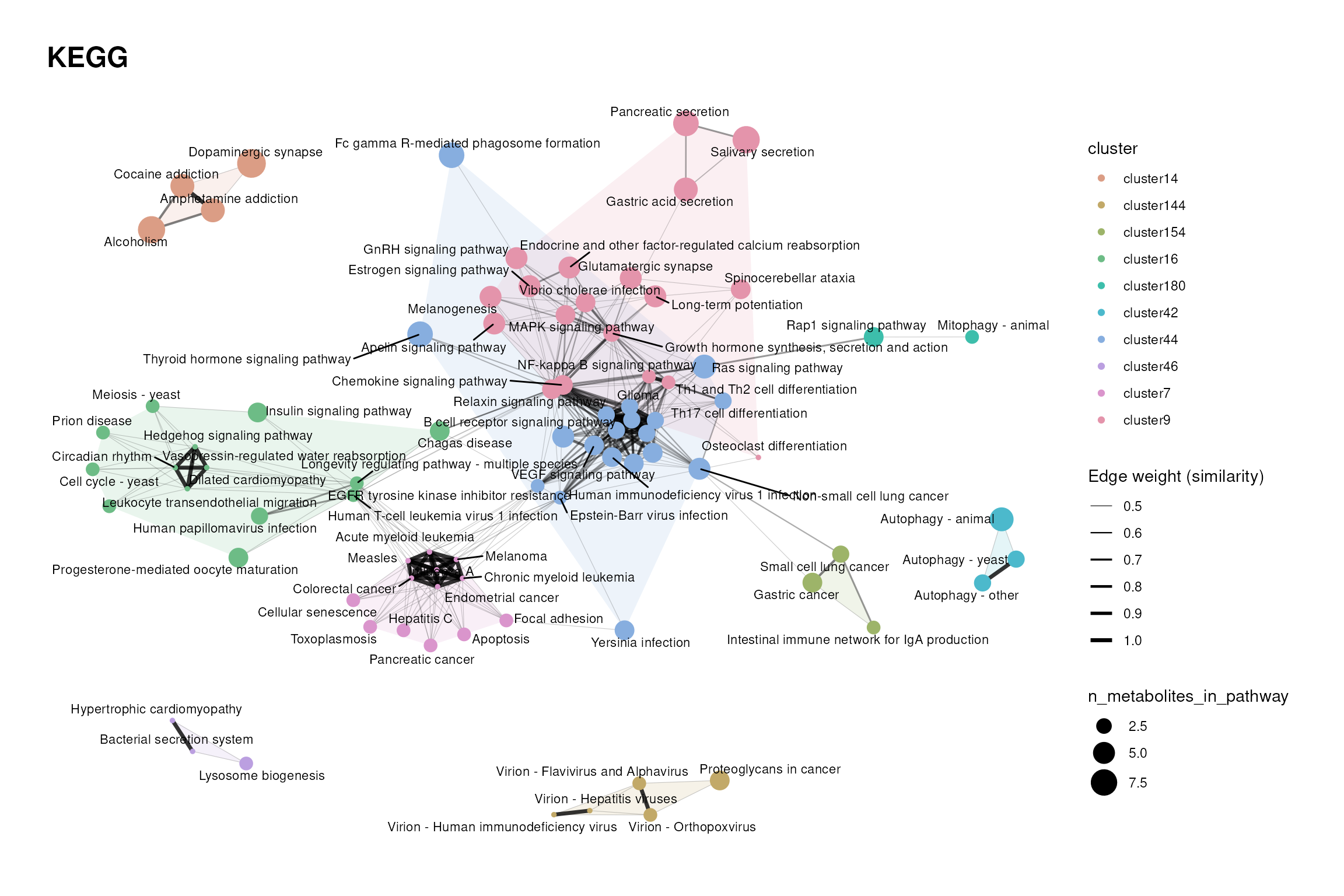
In KEGG, each node is a KEGG pathway and the targets are metabolites (KEGG IDs). KEGG pathways are defined as maps of metabolic reactions, and neighbouring maps share metabolites at their borders, e.g. amino acid degradation pathways that feed into the TCA cycle. We use a strict setting: the Jaccard similarity must be at least 0.4 to form a cluster, and only edges with a similarity of at least 0.5 are drawn. This keeps only pathways that share a large part of their metabolites.

set.seed(123)
kegg_cluster <- cluster_pk(
    kegg,
    metadata_info = c(metabolite_column = "MetaboliteID", pathway_column = "term"),
    similarity = "jaccard",
    input_format = "long",
    threshold = 0.4,
    plot_threshold = 0.5,
    clust = "community",
    min = 2,
    min_degree = 2,
    node_size_column = "n_metabolites_in_pathway",
    show_density = TRUE,
    save_plot = NULL,
    print_plot = TRUE,
    plot_name = "KEGG"
)

scrollable_table(kegg_cluster$cluster_summary, digits = 2, caption = "KEGG cluster summary")

KEGG cluster summary

cluster	n_terms	pct_terms
None	319	70.42
cluster117	2	0.44
cluster125	2	0.44
cluster138	2	0.44
cluster14	4	0.88
cluster144	7	1.55
cluster147	2	0.44
cluster154	3	0.66
cluster16	18	3.97
cluster161	2	0.44
cluster164	2	0.44
cluster178	2	0.44
cluster180	3	0.66
cluster2	2	0.44
cluster227	2	0.44
cluster26	2	0.44
cluster42	4	0.88
cluster44	19	4.19
cluster46	3	0.66
cluster59	2	0.44
cluster66	2	0.44
cluster7	17	3.75
cluster9	32	7.06

The clusters show groups of pathways that share a large part of their metabolites. In an enrichment analysis, pathways of the same cluster are likely to be enriched together, so they should be interpreted as one signal rather than as independent findings. If your data is linked to KEGG, the Prior Knowledge vignette shows how to scale the nodes by the coverage of your measured metabolites instead of the pathway size.

Reactome

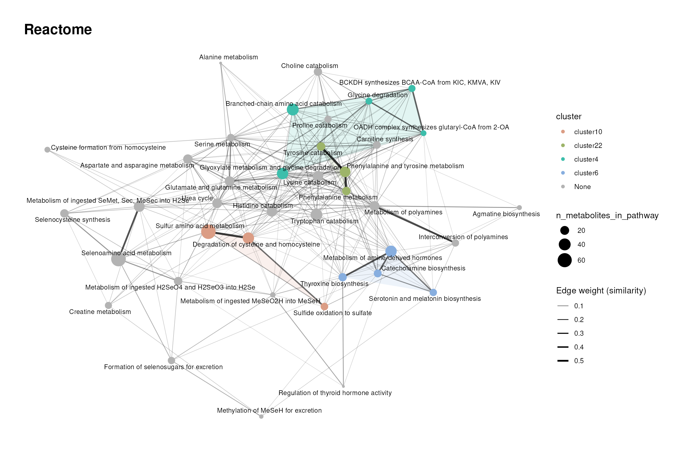
Reactome is organised as a hierarchy: a parent pathway contains all metabolites of its child pathways. Hence, terms of the same branch are nested and similar by design. For the amino acid metabolism subset, we use a looser clustering threshold (0.3), draw weak edges (plot_threshold = 0.1), and only show pathways with at least three connections (min_degree = 3) and clusters of at least four pathways (min = 4) to focus on the densely connected core.

set.seed(123)
reactome_cluster <- cluster_pk(
    reactome,
    metadata_info = c(metabolite_column = "chebi_id", pathway_column = "pathway_name"),
    similarity = "jaccard",
    input_format = "long",
    threshold = 0.3,
    plot_threshold = 0.1,
    clust = "community",
    min = 3,
    min_degree = 4,
    node_size_column = "n_metabolites_in_pathway",
    show_density = TRUE,
    save_plot = NULL,
    print_plot = TRUE,
    plot_name = "Reactome"
)

scrollable_table(reactome_cluster$cluster_summary, digits = 2, caption = "Reactome cluster summary")

Reactome cluster summary

cluster	n_terms	pct_terms
None	27	64.29
cluster10	3	7.14
cluster22	3	7.14
cluster4	5	11.90
cluster6	4	9.52

Since parent and child pathways share most of their metabolites, Reactome enrichment results often list a pathway together with its parents. Clusters help to spot these hierarchies; alternatively, you can restrict the enrichment to one level of the hierarchy.

WikiPathways

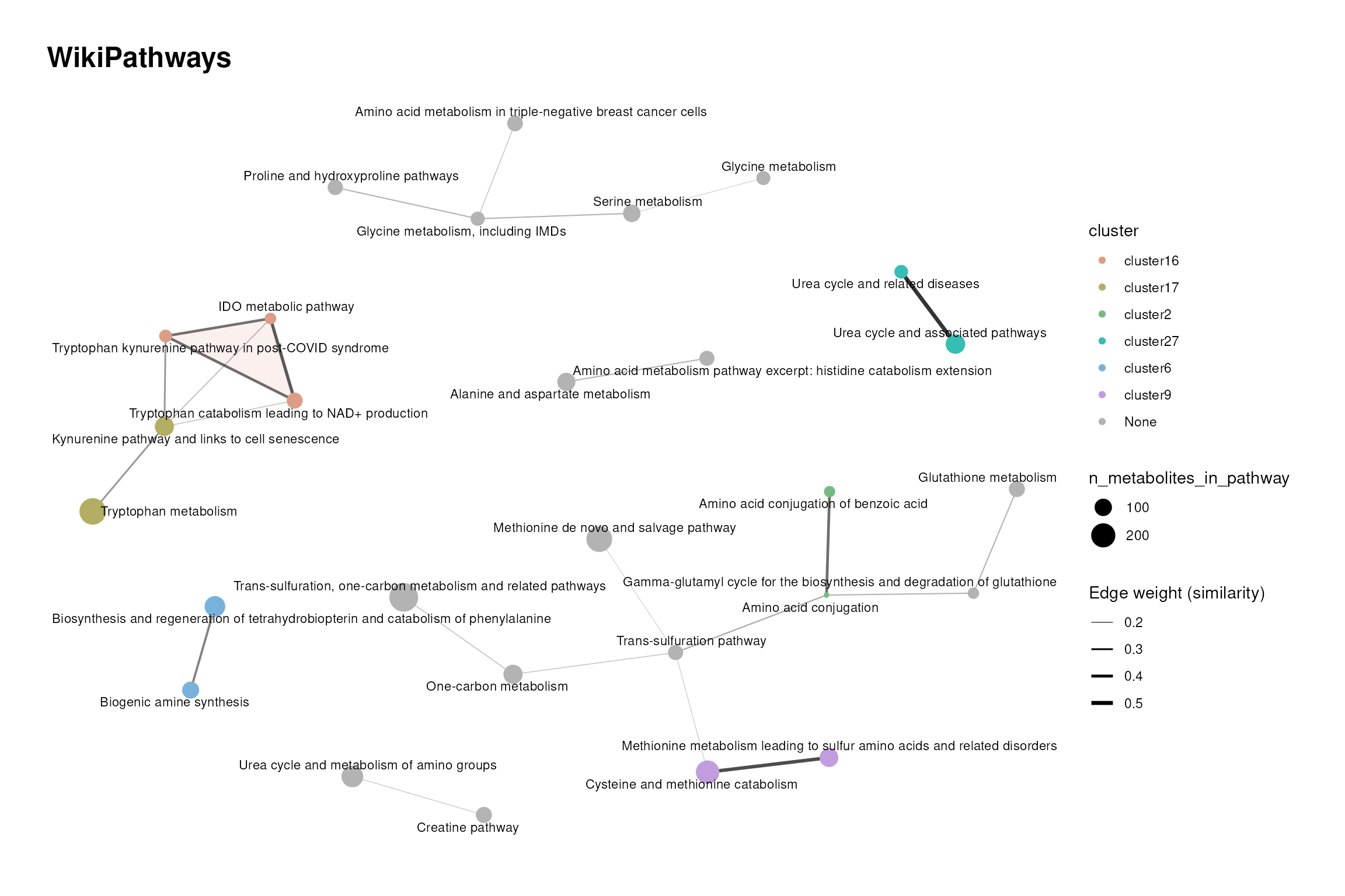
WikiPathways is community curated, and pathways about the same process are often contributed several times with a different focus (e.g. the three urea cycle pathways in our subset). We use a moderate clustering threshold (0.3) and draw edges from a similarity of 0.2.

set.seed(123)
wikipathways_cluster <- cluster_pk(
    wikipathways,
    metadata_info = c(metabolite_column = "hmdb", pathway_column = "pathway_name"),
    similarity = "jaccard",
    input_format = "long",
    threshold = 0.3,
    plot_threshold = 0.2,
    clust = "community",
    min = 2,
    min_degree = 1,
    node_size_column = "n_metabolites_in_pathway",
    show_density = TRUE,
    save_plot = NULL,
    print_plot = TRUE,
    plot_name = "WikiPathways"
)

scrollable_table(wikipathways_cluster$cluster_summary, digits = 2, caption = "WikiPathways cluster summary")

WikiPathways cluster summary

cluster	n_terms	pct_terms
None	22	62.86
cluster16	3	8.57
cluster17	2	5.71
cluster2	2	5.71
cluster27	2	5.71
cluster6	2	5.71
cluster9	2	5.71

Pathways describing the same process end up in the same cluster, whilst pathways with a disease or tissue focus can stand apart, since they contain additional or fewer metabolites. Keep in mind that only metabolites with an HMDB ID after harmonisation (section 1.3) are part of this graph.

MACdb

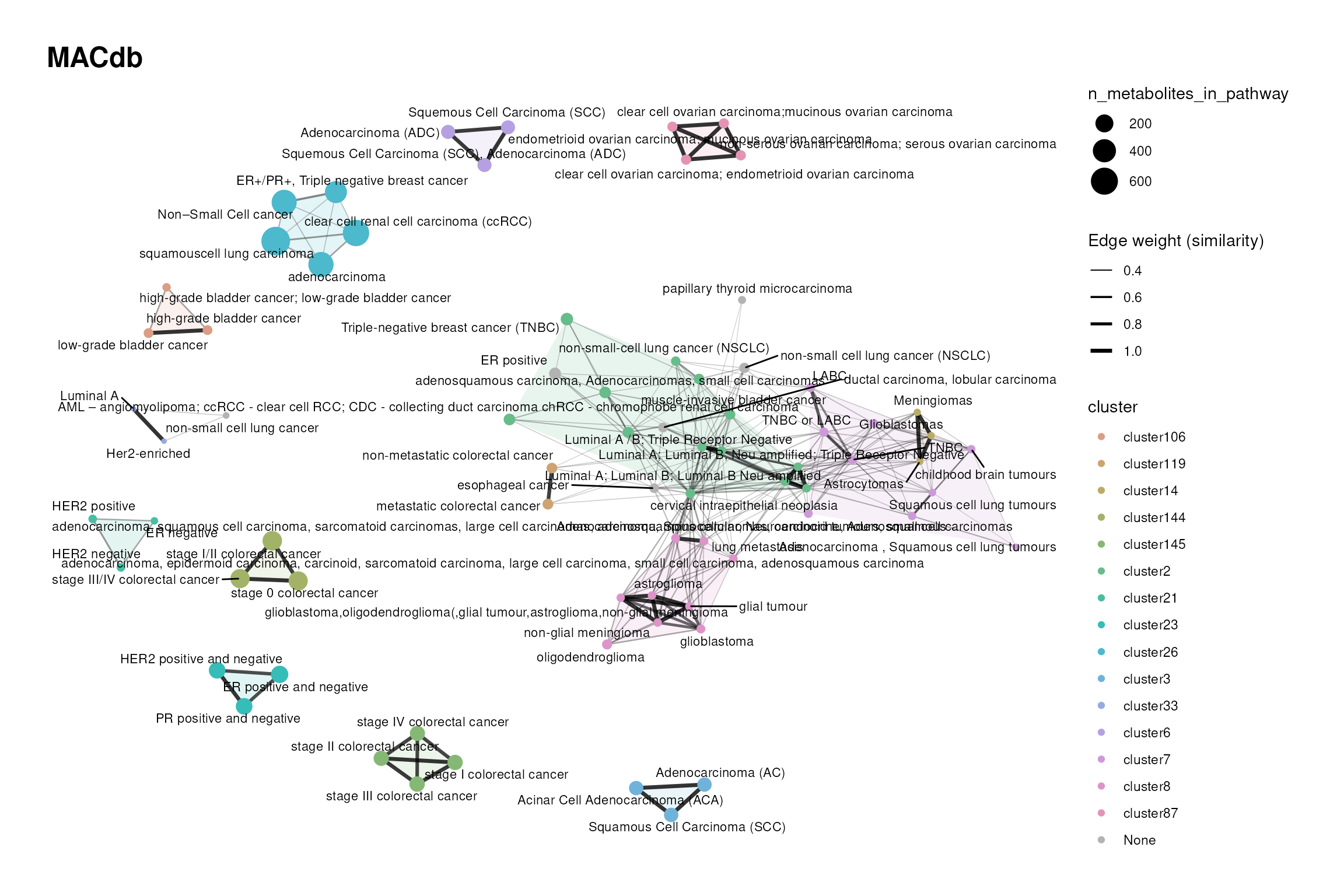
In MACdb, the terms are not pathways but metabolite-cancer associations collected from the literature, and the targets are metabolites (PubChem IDs). Two terms are similar if the same metabolites have been reported as altered in both. We use a strict clustering threshold (0.4) and draw edges from a similarity of 0.3.

set.seed(123)
macdb_cluster <- cluster_pk(
    macdb,
    metadata_info = c(metabolite_column = "Metabolite_PubchemID", pathway_column = "term"),
    similarity = "jaccard",
    input_format = "long",
    threshold = 0.4,
    plot_threshold = 0.3,
    clust = "community",
    min = 2,
    min_degree = 2,
    node_size_column = "n_metabolites_in_pathway",
    show_density = TRUE,
    save_plot = NULL,
    print_plot = TRUE,
    plot_name = "MACdb"
)

scrollable_table(macdb_cluster$cluster_summary, digits = 2, caption = "MACdb cluster summary")

MACdb cluster summary

cluster	n_terms	pct_terms
None	126	59.43
cluster10	2	0.94
cluster100	2	0.94
cluster106	3	1.42
cluster119	2	0.94
cluster138	2	0.94
cluster14	3	1.42
cluster144	3	1.42
cluster145	4	1.89
cluster2	14	6.60
cluster21	3	1.42
cluster23	3	1.42
cluster24	2	0.94
cluster26	5	2.36
cluster3	3	1.42
cluster33	2	0.94
cluster43	2	0.94
cluster5	2	0.94
cluster56	2	0.94
cluster6	3	1.42
cluster7	9	4.25
cluster8	9	4.25
cluster85	2	0.94
cluster87	4	1.89

Clusters can point to cancers with similar reported metabolic alterations. However, the associations depend on which metabolites were measured in the underlying studies, so a cluster can also reflect a shared measurement platform rather than shared biology.

MetaLinks receptor-metabolite

For the MetaLinks subsets, each node is a protein (gene symbol), and the targets are the metabolites it interacts with (HMDB IDs). Two proteins are similar if they interact with the same metabolites, e.g. receptors of the same family that bind the same ligands. This chunk is not evaluated when the vignette is built, because the clustering takes substantially longer than for the other resources. To run it locally, change eval = FALSE to eval = TRUE.

set.seed(123)
receptor_cluster <- cluster_pk(
    receptor,
    metadata_info = c(metabolite_column = "hmdb", pathway_column = "gene_symbol"),
    similarity = "jaccard",
    input_format = "long",
    threshold = 0.4,
    plot_threshold = 0.3,
    clust = "community",
    min = 2,
    min_degree = 2,
    node_size_column = "n_metabolites_in_pathway",
    show_density = TRUE,
    save_plot = NULL,
    print_plot = TRUE,
    plot_name = "MetaLinks receptor"
)
scrollable_table(receptor_cluster$cluster_summary, digits = 2, caption = "MetaLinks receptor cluster summary")

MetaLinks enzyme-metabolite

Here the nodes are metabolic enzymes and the targets are their substrates and products. Enzymes cluster if they act on the same metabolites, e.g. isoenzymes or consecutive steps of a pathway. As for the receptors, this chunk is not evaluated when the vignette is built; change eval = FALSE to eval = TRUE to run it locally.

set.seed(123)
enzyme_cluster <- cluster_pk(
    enzyme,
    metadata_info = c(metabolite_column = "hmdb", pathway_column = "gene_symbol"),
    similarity = "jaccard",
    input_format = "long",
    threshold = 0.4,
    plot_threshold = 0.3,
    clust = "community",
    min = 2,
    min_degree = 2,
    node_size_column = "n_metabolites_in_pathway",
    show_density = TRUE,
    save_plot = NULL,
    print_plot = TRUE,
    plot_name = "MetaLinks enzyme"
)
scrollable_table(enzyme_cluster$cluster_summary, digits = 2, caption = "MetaLinks enzyme cluster summary")

MetaLinks transporter-metabolite

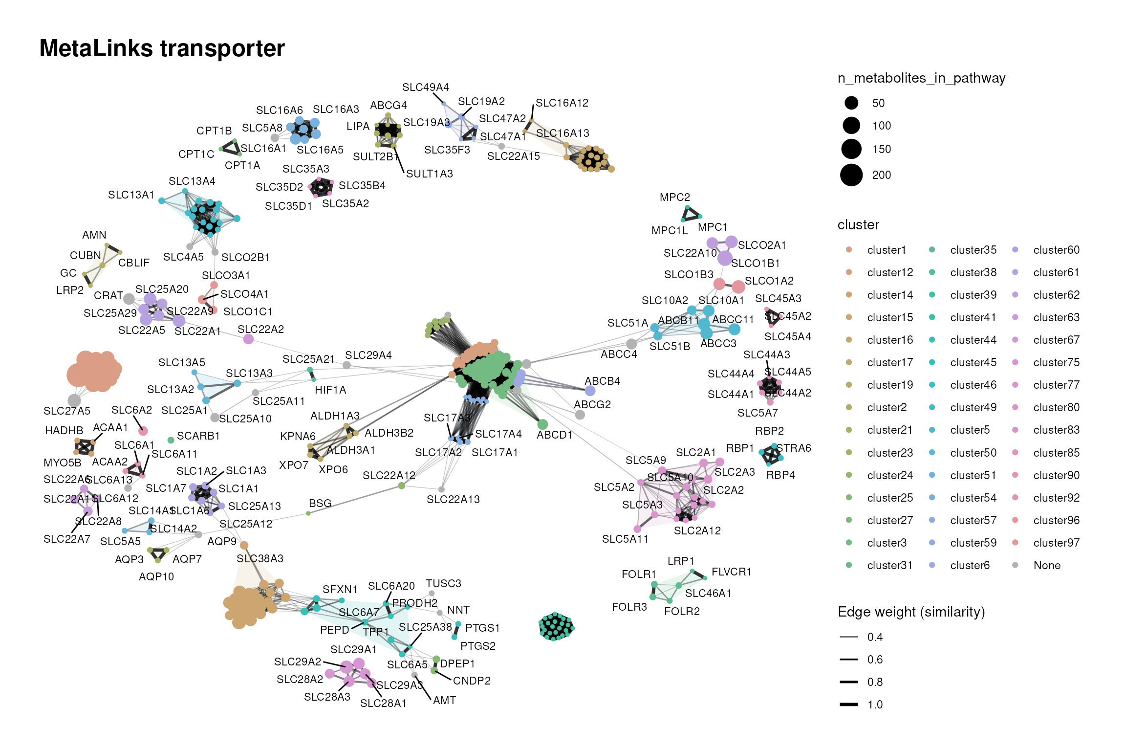
Here the nodes are transporters and the targets are the metabolites they transport. Transporters of the same family often have overlapping substrate profiles, e.g. amino acid transporters.

set.seed(123)
transporter_cluster <- cluster_pk(
    transporter,
    metadata_info = c(metabolite_column = "hmdb", pathway_column = "gene_symbol"),
    similarity = "jaccard",
    input_format = "long",
    threshold = 0.4,
    plot_threshold = 0.3,
    clust = "community",
    min = 2,
    min_degree = 2,
    node_size_column = "n_metabolites_in_pathway",
    show_density = TRUE,
    save_plot = NULL,
    print_plot = TRUE,
    plot_name = "MetaLinks transporter"
)

scrollable_table(transporter_cluster$cluster_summary, digits = 2, caption = "MetaLinks transporter cluster summary")

MetaLinks transporter cluster summary

cluster	n_terms	pct_terms
None	48	9.98
cluster1	16	3.33
cluster12	36	7.48
cluster14	4	0.83
cluster15	28	5.82
cluster16	21	4.37
cluster17	6	1.25
cluster19	5	1.04
cluster2	9	1.87
cluster21	3	0.62
cluster23	7	1.46
cluster24	2	0.42
cluster25	2	0.42
cluster27	3	0.62
cluster3	84	17.46
cluster31	3	0.62
cluster32	2	0.42
cluster35	6	1.25
cluster36	2	0.42
cluster38	2	0.42
cluster39	25	5.20
cluster40	2	0.42
cluster41	3	0.62
cluster44	12	2.49
cluster45	2	0.42
cluster46	4	0.83
cluster49	19	3.95
cluster5	7	1.46
cluster50	4	0.83
cluster51	3	0.62
cluster52	2	0.42
cluster53	2	0.42
cluster54	7	1.46
cluster57	12	2.49
cluster59	6	1.25
cluster6	4	0.83
cluster60	7	1.46
cluster61	6	1.25
cluster62	3	0.62
cluster63	4	0.83
cluster67	2	0.42
cluster71	2	0.42
cluster73	2	0.42
cluster75	6	1.25
cluster77	19	3.95
cluster8	2	0.42
cluster80	5	1.04
cluster83	6	1.25
cluster85	3	0.62
cluster90	3	0.62
cluster92	3	0.62
cluster96	2	0.42
cluster97	3	0.62

Clusters group transporters with similar substrate profiles. In an enrichment analysis on MetaLinks, these transporters would be reported together, since the result is driven by the same metabolites.

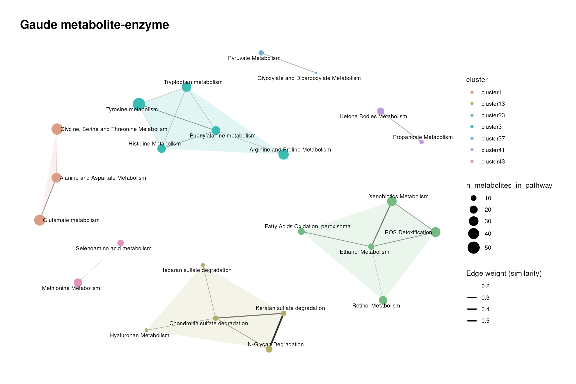
Gaude metabolite-pathway and metabolite-enzyme

Gaude is a collection of metabolic pathways defined by their enzymes (Gaude and Frezza 2018). Through make_gene_metab_set(), each pathway also contains the metabolites of the reactions its enzymes catalyse, and we cluster both parts separately.
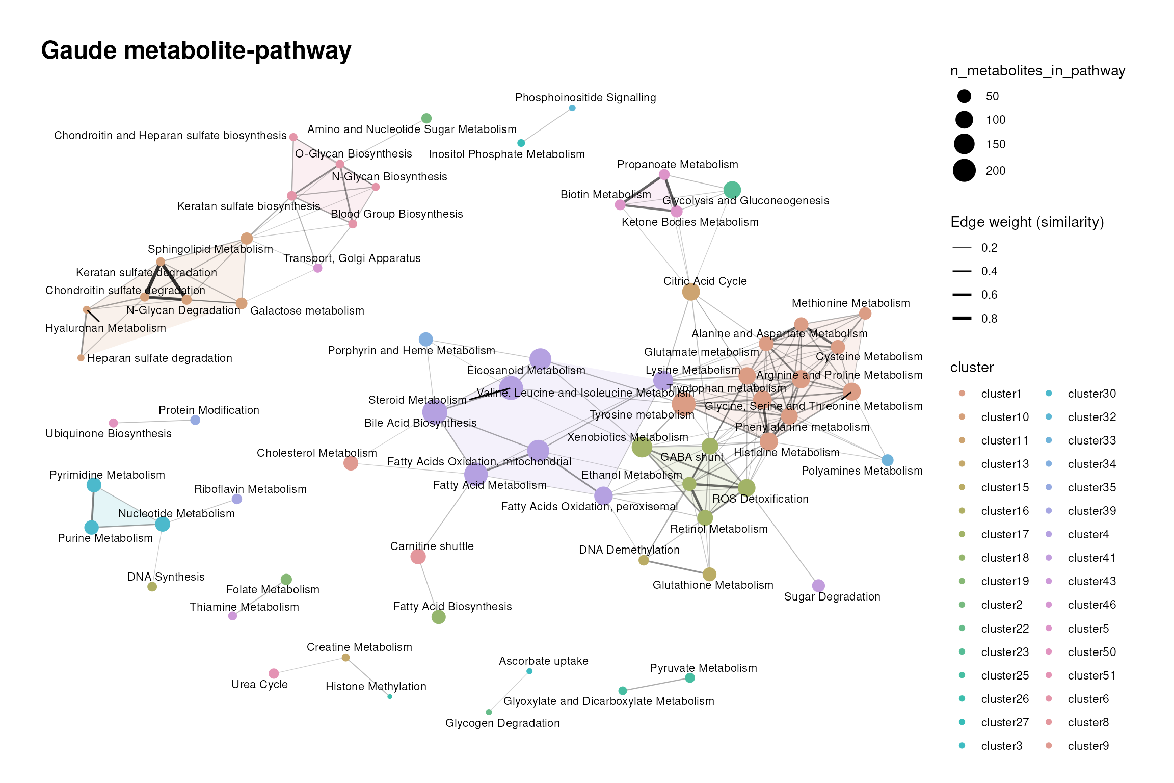
For the metabolite part, we use a moderate threshold (0.3). As the metabolites are assigned via a shared reaction network, metabolites taking part in many reactions connect otherwise different pathways. For the enzyme part, we use a looser threshold (0.2), since pathways defined by enzymes share fewer members.

set.seed(123)
gaude_metabolite_cluster <- cluster_pk(
    gaude_metabolite,
    metadata_info = c(metabolite_column = "target", pathway_column = "term"),
    similarity = "jaccard",
    input_format = "long",
    threshold = 0.3,
    plot_threshold = 0.2,
    clust = "community",
    min = 1,
    min_degree = 1,
    node_size_column = "n_metabolites_in_pathway",
    show_density = TRUE,
    save_plot = NULL,
    print_plot = TRUE,
    plot_name = "Gaude metabolite-pathway"
)

scrollable_table(gaude_metabolite_cluster$cluster_summary, digits = 2, caption = "Gaude metabolite-pathway cluster summary")

Gaude metabolite-pathway cluster summary

cluster	n_terms	pct_terms
cluster1	11	12.22
cluster10	7	7.78
cluster11	1	1.11
cluster12	1	1.11
cluster13	1	1.11
cluster14	1	1.11
cluster15	2	2.22
cluster16	1	1.11
cluster17	5	5.56
cluster18	1	1.11
cluster19	1	1.11
cluster2	1	1.11
cluster20	1	1.11
cluster21	1	1.11
cluster22	1	1.11
cluster23	1	1.11
cluster24	1	1.11
cluster25	2	2.22
cluster26	1	1.11
cluster27	1	1.11
cluster28	1	1.11
cluster29	1	1.11
cluster3	1	1.11
cluster30	3	3.33
cluster31	1	1.11
cluster32	1	1.11
cluster33	1	1.11
cluster34	1	1.11
cluster35	1	1.11
cluster36	1	1.11
cluster37	1	1.11
cluster38	1	1.11
cluster39	1	1.11
cluster4	7	7.78
cluster40	1	1.11
cluster41	1	1.11
cluster42	1	1.11
cluster43	1	1.11
cluster44	1	1.11
cluster45	1	1.11
cluster46	1	1.11
cluster47	1	1.11
cluster48	1	1.11
cluster49	1	1.11
cluster5	3	3.33
cluster50	1	1.11
cluster51	1	1.11
cluster52	1	1.11
cluster53	1	1.11
cluster54	1	1.11
cluster6	5	5.56
cluster7	1	1.11
cluster8	1	1.11
cluster9	1	1.11

set.seed(123)
gaude_enzyme_cluster <- cluster_pk(
    gaude_enzyme,
    metadata_info = c(metabolite_column = "target", pathway_column = "term"),
    similarity = "jaccard",
    input_format = "long",
    threshold = 0.2,
    plot_threshold = 0.2,
    clust = "community",
    min = 1,
    min_degree = 1,
    node_size_column = "n_metabolites_in_pathway",
    show_density = TRUE,
    save_plot = NULL,
    print_plot = TRUE,
    plot_name = "Gaude metabolite-enzyme"
)

scrollable_table(gaude_enzyme_cluster$cluster_summary, digits = 2, caption = "Gaude metabolite-enzyme cluster summary")

Gaude metabolite-enzyme cluster summary

cluster	n_terms	pct_terms
cluster1	3	3.12
cluster10	1	1.04
cluster11	1	1.04
cluster12	1	1.04
cluster13	5	5.21
cluster14	1	1.04
cluster15	1	1.04
cluster16	1	1.04
cluster17	1	1.04
cluster18	1	1.04
cluster19	1	1.04
cluster2	1	1.04
cluster20	1	1.04
cluster21	1	1.04
cluster22	1	1.04
cluster23	5	5.21
cluster24	1	1.04
cluster25	1	1.04
cluster26	1	1.04
cluster27	1	1.04
cluster28	1	1.04
cluster29	1	1.04
cluster3	5	5.21
cluster30	1	1.04
cluster31	1	1.04
cluster32	1	1.04
cluster33	1	1.04
cluster34	1	1.04
cluster35	1	1.04
cluster36	1	1.04
cluster37	2	2.08
cluster38	1	1.04
cluster39	1	1.04
cluster4	1	1.04
cluster40	1	1.04
cluster41	2	2.08
cluster42	1	1.04
cluster43	2	2.08
cluster44	1	1.04
cluster45	1	1.04
cluster46	1	1.04
cluster47	1	1.04
cluster48	1	1.04
cluster49	1	1.04
cluster5	1	1.04
cluster50	1	1.04
cluster51	1	1.04
cluster52	1	1.04
cluster53	1	1.04
cluster54	1	1.04
cluster55	1	1.04
cluster56	1	1.04
cluster57	1	1.04
cluster58	1	1.04
cluster59	1	1.04
cluster6	1	1.04
cluster60	1	1.04
cluster61	1	1.04
cluster62	1	1.04
cluster63	1	1.04
cluster64	1	1.04
cluster65	1	1.04
cluster66	1	1.04
cluster67	1	1.04
cluster68	1	1.04
cluster69	1	1.04
cluster7	1	1.04
cluster70	1	1.04
cluster71	1	1.04
cluster72	1	1.04
cluster73	1	1.04
cluster74	1	1.04
cluster75	1	1.04
cluster76	1	1.04
cluster77	1	1.04
cluster78	1	1.04
cluster79	1	1.04
cluster8	1	1.04
cluster9	1	1.04

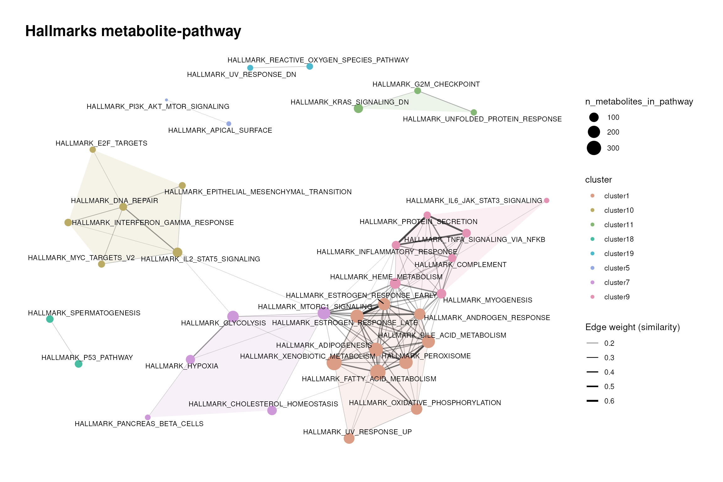
Comparing both graphs shows how much of the redundancy is introduced by the metabolite assignment: pathways that are separate on the enzyme level can be connected on the metabolite level.

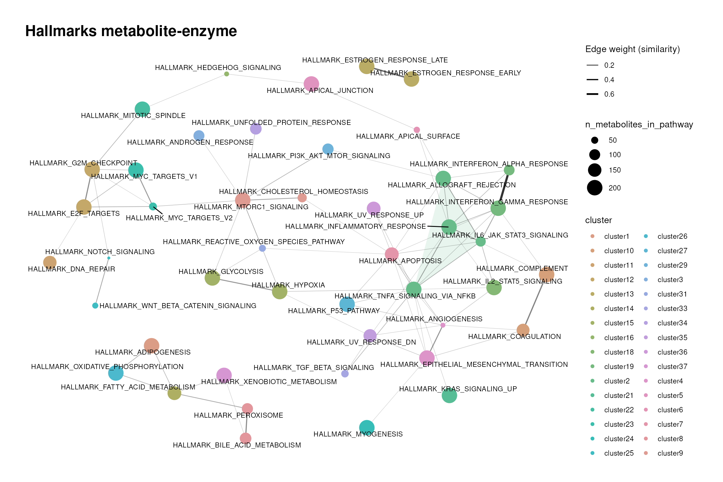
Hallmarks metabolite-pathway and metabolite-enzyme

The Hallmarks are 50 gene-sets that summarise well-defined biological states or processes (Liberzon et al. 2015). Most of them are not metabolic, so only the metabolic enzymes of each gene-set (and their metabolites) remain after make_gene_metab_set().
For the metabolite part, we use a loose threshold (0.2). For the enzyme part, the remaining enzyme sets are small and partially nested, hence we use the overlap coefficient instead of the Jaccard similarity, with a threshold of 0.25, and draw edges from a similarity of 0.1. This is the loosest setting in this vignette.

set.seed(123)
hallmarks_metabolite_cluster <- cluster_pk(
    hallmarks_metabolite,
    metadata_info = c(metabolite_column = "target", pathway_column = "term"),
    similarity = "jaccard",
    input_format = "long",
    threshold = 0.2,
    plot_threshold = 0.2,
    clust = "community",
    min = 1,
    min_degree = 1,
    node_size_column = "n_metabolites_in_pathway",
    show_density = TRUE,
    save_plot = NULL,
    print_plot = TRUE,
    plot_name = "Hallmarks metabolite-pathway"
)

scrollable_table(hallmarks_metabolite_cluster$cluster_summary, digits = 2, caption = "Hallmarks metabolite-pathway cluster summary")

Hallmarks metabolite-pathway cluster summary

cluster	n_terms	pct_terms
cluster1	10	20.83
cluster10	6	12.50
cluster11	3	6.25
cluster12	1	2.08
cluster13	1	2.08
cluster14	1	2.08
cluster15	1	2.08
cluster16	1	2.08
cluster17	1	2.08
cluster18	2	4.17
cluster19	2	4.17
cluster2	1	2.08
cluster3	1	2.08
cluster4	1	2.08
cluster5	2	4.17
cluster6	1	2.08
cluster7	5	10.42
cluster8	1	2.08
cluster9	7	14.58

set.seed(123)
hallmarks_enzyme_cluster <- cluster_pk(
    hallmarks_enzyme,
    metadata_info = c(metabolite_column = "target", pathway_column = "term"),
    similarity = "overlap_coefficient",
    input_format = "long",
    threshold = 0.25,
    plot_threshold = 0.1,
    clust = "community",
    min = 1,
    min_degree = 1,
    node_size_column = "n_metabolites_in_pathway",
    show_density = TRUE,
    save_plot = NULL,
    print_plot = TRUE,
    plot_name = "Hallmarks metabolite-enzyme"
)

scrollable_table(hallmarks_enzyme_cluster$cluster_summary, digits = 2, caption = "Hallmarks metabolite-enzyme cluster summary")

Hallmarks metabolite-enzyme cluster summary

cluster	n_terms	pct_terms
cluster1	1	2
cluster10	2	4
cluster11	1	2
cluster12	2	4
cluster13	2	4
cluster14	1	2
cluster15	2	4
cluster16	1	2
cluster17	1	2
cluster18	1	2
cluster19	2	4
cluster2	4	8
cluster20	1	2
cluster21	1	2
cluster22	1	2
cluster23	2	4
cluster24	1	2
cluster25	2	4
cluster26	1	2
cluster27	1	2
cluster28	1	2
cluster29	1	2
cluster3	1	2
cluster30	1	2
cluster31	1	2
cluster32	1	2
cluster33	1	2
cluster34	1	2
cluster35	1	2
cluster36	1	2
cluster37	1	2
cluster4	2	4
cluster5	1	2
cluster6	1	2
cluster7	1	2
cluster8	2	4
cluster9	2	4

Hallmarks that share metabolic enzymes (e.g. glycolysis and hypoxia) end up close to each other. Since the overlap coefficient rates a small set nested in a larger one as fully similar, these clusters should be read as “shares its metabolic part with” rather than “is the same as”.

Choosing a resource

There is no single best resource. Based on the composition and clustering results, we suggest to consider the following questions:

• Which question do you ask? Pathways (KEGG, Reactome, WikiPathways) for metabolic processes, ClassyFire for chemical classes, MetaLinks for metabolite-protein interactions, MACdb for comparison to reported cancer alterations, and Gaude or Hallmarks for a joint analysis with transcriptomics or proteomics data.
• Which IDs do you have? Each resource uses one ID type (section 1.2). If your data uses another type, use translate_id() and check the mapping ambiguity, as shown in the Prior Knowledge vignette.
• How large are the terms? Small terms are specific but may not be covered by your measured metabolites; large terms are nearly always covered but less informative (section 2.2).
• How redundant are the terms? In resources with recurrent targets and dense clusters, expect groups of enriched terms that describe the same signal (sections 2.3 and 3).
• Which metabolites are excluded? Use the same exclusion for the resource and for the metabolite universe of your enrichment analysis (section 2.4).

Session information

#> R version 4.6.1 (2026-06-24)
#> Platform: x86_64-pc-linux-gnu
#> Running under: Ubuntu 24.04.4 LTS
#> 
#> Matrix products: default
#> BLAS:   /usr/lib/x86_64-linux-gnu/openblas-pthread/libblas.so.3 
#> LAPACK: /usr/lib/x86_64-linux-gnu/openblas-pthread/libopenblasp-r0.3.26.so;  LAPACK version 3.12.0
#> 
#> locale:
#>  [1] LC_CTYPE=en_US.UTF-8       LC_NUMERIC=C               LC_TIME=en_US.UTF-8        LC_COLLATE=en_US.UTF-8    
#>  [5] LC_MONETARY=en_US.UTF-8    LC_MESSAGES=en_US.UTF-8    LC_PAPER=en_US.UTF-8       LC_NAME=C                 
#>  [9] LC_ADDRESS=C               LC_TELEPHONE=C             LC_MEASUREMENT=en_US.UTF-8 LC_IDENTIFICATION=C       
#> 
#> time zone: Etc/UTC
#> tzcode source: system (glibc)
#> 
#> attached base packages:
#> [1] stats     graphics  grDevices utils     datasets  methods   base     
#> 
#> other attached packages:
#> [1] scales_1.4.0      knitr_1.52        ggplot2_4.0.3     tibble_3.3.1      purrr_1.2.2       tidyr_1.3.2      
#> [7] dplyr_1.2.1       MetaProViz_4.99.0 BiocStyle_2.40.0 
#> 
#> loaded via a namespace (and not attached):
#>   [1] splines_4.6.1               later_1.4.8                 R.oo_1.27.1                 cellranger_1.1.0           
#>   [5] polyclip_1.10-7             XML_3.99-0.25               factoextra_2.2.0            lifecycle_1.0.5            
#>   [9] httr2_1.3.0                 tcltk_4.6.1                 rstatix_1.1.0               lattice_0.22-9             
#>  [13] vroom_1.7.1                 MASS_7.3-66                 backports_1.5.1             magrittr_2.0.5             
#>  [17] limma_3.68.5                sass_0.4.10                 rmarkdown_2.32              jquerylib_0.1.4            
#>  [21] yaml_2.3.12                 otel_0.2.0                  zip_3.0.2                   sessioninfo_1.2.4          
#>  [25] EnhancedVolcano_1.31.0      DBI_1.3.0                   RColorBrewer_1.1-3          lubridate_1.9.5            
#>  [29] abind_1.4-8                 rvest_1.0.5                 GenomicRanges_1.64.0        R.utils_2.13.0             
#>  [33] ggraph_2.2.2                BiocGenerics_0.58.1         hash_2.2.6.4                tweenr_2.0.3               
#>  [37] rappdirs_0.3.4              IRanges_2.46.0              S4Vectors_0.50.3            ggrepel_0.9.8              
#>  [41] pheatmap_1.0.13             parallelly_1.48.0           pkgdown_2.2.1               svglite_2.2.2              
#>  [45] codetools_0.2-20            DelayedArray_0.38.2         xml2_1.6.0                  ggforce_0.5.0              
#>  [49] tidyselect_1.2.1            farver_2.1.2                viridis_0.6.5               ComplexUpset_1.3.3         
#>  [53] matrixStats_1.5.0           stats4_4.6.1                Seqinfo_1.2.0               jsonlite_2.0.0             
#>  [57] tidygraph_1.3.1             Formula_1.2-6               systemfonts_1.3.2           tools_4.6.1                
#>  [61] progress_1.2.3              ragg_1.5.2                  Rcpp_1.1.2                  glue_1.8.1                 
#>  [65] gridExtra_2.3.1             SparseArray_1.12.3          xfun_0.61                   decoupleR_2.17.0           
#>  [69] qvalue_2.44.0               MatrixGenerics_1.24.0       ggfortify_0.4.24            withr_3.0.3                
#>  [73] BiocManager_1.30.27         fastmap_1.2.0               digest_0.6.39               timechange_0.4.0           
#>  [77] R6_2.6.1                    textshaping_1.0.5           colorspace_2.1-3            lpSolve_5.6.23             
#>  [81] gtools_3.9.5                RSQLite_3.53.3              R.methodsS3_1.8.2           generics_0.1.4             
#>  [85] prettyunits_1.2.0           graphlayouts_1.2.5          httr_1.4.9                  htmlwidgets_1.6.4          
#>  [89] S4Arrays_1.12.1             scatterplot3d_0.3-45        inflection_1.3.7            pkgconfig_2.0.3            
#>  [93] gtable_0.3.6                blob_1.3.0                  S7_0.2.2                    XVector_0.52.0             
#>  [97] OmnipathR_4.1.0             htmltools_0.5.9             carData_3.0-6               bookdown_0.48              
#> [101] kableExtra_1.4.1            Biobase_2.72.0              rstudioapi_0.19.0           tzdb_0.5.0                 
#> [105] reshape2_1.4.5              rjson_0.2.23                checkmate_2.3.4             curl_8.0.0                 
#> [109] cachem_1.1.0                Polychrome_1.6.2            stringr_1.6.0               parallel_4.6.1             
#> [113] vipor_0.4.7                 cosmosR_1.20.0              desc_1.4.3                  pillar_1.11.1              
#> [117] grid_4.6.1                  logger_0.4.3                vctrs_0.7.3                 ggpubr_1.0.0               
#> [121] car_3.1-5                   beeswarm_0.4.0              evaluate_1.0.5              readr_2.2.0                
#> [125] cli_3.6.6                   compiler_4.6.1              rlang_1.3.0                 crayon_1.5.3               
#> [129] ggsignif_0.6.4              labeling_0.4.3              plyr_1.8.9                  fs_2.1.0                   
#> [133] ggbeeswarm_0.7.3            writexl_2.0.1               stringi_1.8.9               viridisLite_0.4.3          
#> [137] BiocParallel_1.46.0         Matrix_1.7-6                hms_1.1.4                   patchwork_1.3.2            
#> [141] bit64_4.8.6                 statmod_1.5.2               SummarizedExperiment_1.42.0 CARNIVAL_2.22.0            
#> [145] igraph_2.3.4                broom_1.0.13                memoise_2.0.1               bslib_0.12.0               
#> [149] bit_4.6.0                   readxl_1.5.0.1

Bibliography

Agrawal, A et al. 2024. “WikiPathways 2024: Next Generation Pathway Database.” Nucleic Acids Research 52.

Djoumbou Feunang, Yannick et al. 2016. “ClassyFire: Automated Chemical Classification.” Journal of Cheminformatics 8: 61.

Farr, E et al. 2024. “MetaLinks: A Database of Metabolite–Protein Interactions.” Nucleic Acids Research.

Gaude, Edoardo, and Christian Frezza. 2018. “Metabolic Pathways in Cancer.” Nature Reviews Cancer 18: 619–34.

Kanehisa, Minoru et al. 2017. “KEGG: New Perspectives on Genomes, Pathways, Diseases and Drugs.” Nucleic Acids Research 45: D353–61.

Liberzon, Arthur et al. 2015. “The Molecular Signatures Database Hallmark Gene Set Collection.” Cell Systems 1: 417–25.

Milacic, Marija et al. 2024. “The Reactome Pathway Knowledgebase 2024.” Nucleic Acids Research 52: D672–78.

Sun, Y et al. 2023. “MACdb: A Database of Metabolite Associations with Cancer.” Nucleic Acids Research.