CoRe Metabolomics

Christina Schmidt

Heidelberg University

Dimitrios Prymidis

Cologne University

A Consumption-Release (core) metabolomics experiment usually refers to a cell culture experiment where metabolomics is performed on the cell culture media.

In this tutorial we showcase how to use MetaProViz:

• to process raw peak data and identify outliers.
  
• to perform differential metabolite analysis (dma) to generate Log2Distance and statistics and perform pathway analysis using Over Representation Analysis (ORA) on the results.
  
• to do metabolite clustering analysis (MCA) to find clusters of metabolites with similar behaviors and perform pathway analysis using ORA on each cluster.
  
• to use specific visualizations to aid biological interpretation of the results.
  

First if you have not done yet, install the required dependencies and load the libraries:

# 1. Install MetaProViz from Bioconductor devel:
# if (!requireNamespace("BiocManager", quietly = TRUE)) install.packages("BiocManager")
# BiocManager::install(version = "devel")
# BiocManager::install("MetaProViz")
# 2. Install the latest development version from GitHub using devtools
# remotes::install_github("saezlab/MetaProViz") # Install Rtools if you haven’t done this yet, using the appropriate version (e.g.windows or macOS).

library(MetaProViz)

# dependencies that need to be loaded:
library(magrittr)
library(dplyr)
library(tibble)
library(rlang)
library(ggfortify)
library(stringr)
library(tibble)

Loading the example data

Here we choose an example dataset, which is publicly available on metabolomics workbench project PR001418 including metabolic profiles of human renal epithelial cells HK2 and cell renal cell carcinoma (ccRCC) cell lines cultured in Plasmax cell culture media. Here we use the integrated raw peak data as example data using the trivial metabolite name in combination with the KEGG ID as the metabolite identifiers.

As part of the MetaProViz package you can load the example data into your global environment using data():

1. core experiment (core)
The raw data are available via metabolomics workbench study ST002226 where exometabolomics of HK2 and ccRCC cell lines 786-O, 786-M1A, 786-M2A, OS-RC-2, OS-LM1 and RFX-631 were performed.

data(medium_raw)

Media <- medium_raw%>%
column_to_rownames("Code")

Preview of the DF core including columns with sample information and metabolite ids with their measured values.

	Conditions	Biological_Replicates	GrowthFactor	valine-d8	hipppuric acid-d5	2-hydroxyglutarate	2-ketoglutarate	3-Dehydro-L-threonate
MS51-06	HK2	1	249.2817	780552871	3127630257	84950547	169244158	1807489245
MS51-07	HK2	2	249.2817	802602348	3256031922	60753859	151064767	695228424
MS51-08	HK2	3	249.2817	831984796	3308009345	73718363	171281531	791442407
MS51-09	HK2	4	249.2817	822744518	3209731571	65933166	112033043	315209589
MS51-10	HK2	5	249.2817	805565867	3297793480	68183576	170902744	615035216
MS51-11	786-O	1	297.3423	841873509	3418515398	75941661	215553005	501977089
MS51-12	786-O	2	297.3423	825462964	3218049751	62100210	195308040	484681099

2. Additional information mapping the trivial metabolite names to KEGG IDs and selected pathways (MappingInfo)

data(cellular_meta)

MappingInfo <- cellular_meta%>%
column_to_rownames("Metabolite")

Preview of the DF Pathways including the trivial metabolite identifiers used in the experiment as well as KEGG IDs and pathway information.

	HMDB	KEGG.ID	KEGGCompound	Pathway
N-acetylaspartate	HMDB0000812	C01042	N-Acetyl-L-aspartate	Alanine, aspartate and glutamate metabolism
argininosuccinate	HMDB0000052	C03406	N-(L-Arginino)succinate	Alanine, aspartate and glutamate metabolism
N-acetylaspartylglutamate	HMDB0001067	C12270	N-Acetylaspartylglutamate	Alanine, aspartate and glutamate metabolism
tyrosine	HMDB0000158	C00082	L-Tyrosine	Amino acid metabolism
asparagine	HMDB0000168	C00152	L-Asparagine	Amino acid metabolism

3. KEGG pathways that are loaded from the KEGG API via OmnipathR and can be used to perform pathway analysis. (KEGG_Pathways)

# This queries the KEGG API (via OmnipathR) to load the pathways:
KEGG_Pathways <- metsigdb_kegg()

Preview of the DF KEGG_Pathways.

Description	MetaboliteID	term	Metabolite	pubchem	compound_names
map00010	C00022	Glycolysis / Gluconeogenesis	Pyruvate	3324	Pyruvate….
map00010	C00024	Glycolysis / Gluconeogenesis	Acetyl-CoA	3326	Acetyl-C….
map00010	C00031	Glycolysis / Gluconeogenesis	D-Glucose	3333	D-Glucos….
map00010	C00033	Glycolysis / Gluconeogenesis	Acetate	3335	Acetate,….
map00010	C00036	Glycolysis / Gluconeogenesis	Oxaloacetate	3338	Oxaloace….

Run MetaProViz Analysis

Currently, MetaProViz contains four different modules, which include different methods and can be used independently from each other or in combination (see introduction for more details). Here we will go through each of those modules and apply them to the example data.

Pre-processing

MetaProViz includes a pre-processing module with the function processing() that has multiple parameters to perform customize data processing.
featurefilt applies the 80%-filtering rule on the metabolite features either on the whole dataset (=“Standard”) (Bijlsma et al. 2006) or per condition (=“Modified”) (Wei et al. 2018). This means that metabolites are removed where more than 20% of the samples (all or per condition) have no detection. In case of the core experiment, the blank samples are ignored during feature filtering, since often metabolites are released from a cell and not naturally present in the culture media leading to no detection in the blank. With the parameter cutoff_featurefilt we enable the adaptation of the stringency of the filtering based on the experimental context. For instance, patient tumour samples can contain many unknown subgroups due to gender, age, stage etc., which leads to a metabolite being detected in only 50% (or even less) of the tumour samples, hence in this context it could be considered to change the cutoff_featurefilt from the default (=0.8). If featurefilt = NULL, no feature filtering is performed. In the context of featurefilt it is also noteworthy that the function pool_estimation() can be used to estimate the quality of the metabolite detection and will return a list of metabolites that are variable across the different pool measurements (pool = mixture of all experimental samples measured several times during the LC-MS run) . Variable metabolite in the pool sample should be removed from the data.
The parameter tic refers to total Ion Count (tic) normalisation, which is often used with LC-MS derived metabolomics data. If tic = TRUE, each feature (=metabolite) in a sample is divided by the sum of all intensity value (= total number of ions) for the sample and finally multiplied by a constant ( = the mean of all samples total number of ions). Noteworthy, tic normalisation should not be used with small number of features (= metabolites), since tic assumes that on “average” the ion count of each sample is equal if there were no instrument batch effects (Wulff and Mitchell 2018).
The parameter mvi refers to Missing Value Imputation (mvi) and if mvi = TRUE half minimum (HM) missing value imputation is performed per feature (= per metabolite). Here it is important to mention that HM has been shown to perform well for missing values that are missing not at random (MNAR) (Wei et al. 2018).
Lastly, the function processing() performs outlier detection and adds a column “Outliers” into the DF, which can be used to remove outliers. The parameter hotellins_confidence can be used to choose the confidence interval that should be used for the Hotelling’s T2 outlier test (Hotelling 1931).

Since our example data contains pool samples, we will do pool_estimation() before applying the processing() function. This is important, since one should remove the features (=metabolites) that are too variable prior to performing any data transformations such as tic as part of the processing() function.
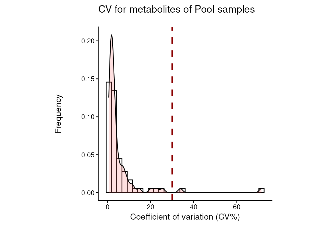
It is worth mentioning that the Coefficient of variation (CV) is calculated by dividing the standard deviation (SD) by the mean. Hence CV depends on the SD, which in turn works for normally distributed data.

Pool_Estimation_result<- pool_estimation(data = Media[,-c(1:3)],
                                                    metadata_sample = Media[,1:3],
                                                    metadata_info = c(PoolSamples = "Pool", Conditions="Conditions"),
                                                    cutoff_cv = 30)
#> `stat_bin()` using `bins = 30`. Pick better value `binwidth`.
#> Bin width defaults to 1/30 of the range of the data. Pick better value with
#> `binwidth`.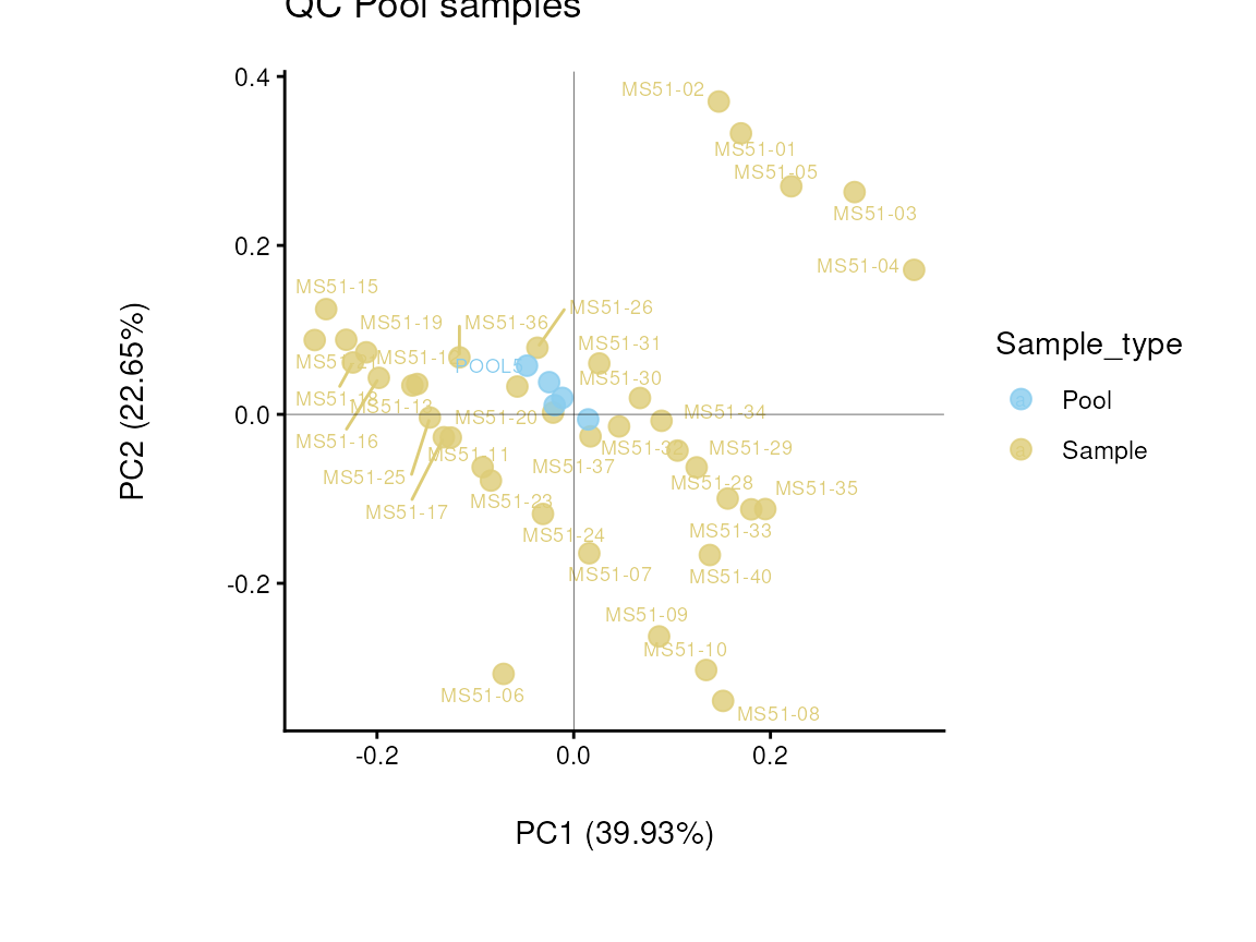

Pool_Estimation_result_DF_CV <-Pool_Estimation_result[["DF"]][["CV"]]

Preview of the Pool_Estimation result.

Metabolite	CV	HighVar	MissingValuepercentage
valine-d8	1.744198	FALSE	0
hipppuric acid-d5	1.253983	FALSE	0
2-hydroxyglutarate	7.199141	FALSE	0
2-ketoglutarate	2.766989	FALSE	0
3-Dehydro-L-threonate	9.222780	FALSE	0

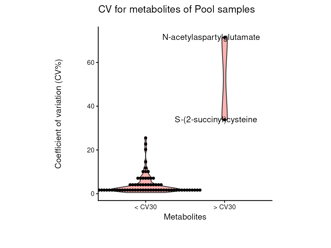
The results from the pool_estimation() is a table that has the CVs. If there is a high variability, one should consider to remove those features from the data. For the example data nothing needs to be removed. If you have used internal standard in your experiment you should specifically check their CV as this would indicate technical issues (here valine-d8 and hippuric acid-d5).

Now we will apply the processing() function to the example data and have a look at the output produced. You will notice that all the chosen parameters and results are documented in messages. All the results data tables, the Quality Control (QC) plots and outlier detection plots are returned and can be easily viewed. Importantly, here we are able to specify that we have a core experiment setting the parameter core=TRUE, in which case a few additional data processing steps are applied:
1. Blank sample: This refers to media samples where no cells have been cultured in, which will be used as blank. In detail, the mean of the blank sample of a feature (= metabolite) will be subtracted from the values measured in each sample for the same feature. In the column “Conditions” of metadata_sample, you will need to label your blank samples with “blank”.
2. Growth factor or growth rate: This refers to the different conditions and is either based on cell count or protein quantification at the start of the experiment (t0) and at the end of the experiment (t1) resulting in the growth factor (t0/t1). Otherwise, one can experimentally estimate the growth rate of each condition. Ultimately, this measure is used to normalize the data, since the amount of growth will impact the consumption and release of metabolites from the media and hence we need to account for this. If you do not have this information, this will be set to 1, yet be aware that this may affect the results.

You can pass this additional information via the parameter metadata_info, by passing the column name of the growth factor in metadata_sample as core_norm_factor and the condition name of the blank samples as core_media.

# Prepare the input:
Media_input <- Media%>%
subset(!Conditions=="Pool", select = -c(1:3))#remove pool samples and remove the information columns

Media_Metadata <- Media%>%
subset(!Conditions=="Pool", select = c(1:3))#remove pool samples and keep the information columns only

PreProcessing_res <-  processing(data=Media_input,
                                                metadata_sample =Media_Metadata,
                                                metadata_info = c(Conditions = "Conditions",
                                                Biological_Replicates = "Biological_Replicates",
                                                core_norm_factor = "GrowthFactor",
                                                core_media = "blank"),
                                                featurefilt = "Modified",
                                                cutoff_featurefilt = 0.8,
                                                tic = TRUE,# As we have raw data we will perform total ion count norm
                                                mvi=TRUE, #We assume the values are not missing at random and perform half minimum mvi
                                                mvi_percentage=50,
                                                hotellins_confidence = 0.99,# We perform outlier testing using 0.99 confidence interval
                                                core = TRUE)
#> For Consumption Release experiment we are using the method from Jain M.  REF: Jain et. al, (2012), Science 336(6084):1040-4, doi: 10.1126/science.1218595.
#> feature_filtering: Here we apply the modified 80%-filtering rule that takes the class information (Column `Conditions`) into account, which additionally reduces the effect of missing values (REF: Yang et. al., (2015), doi: 10.3389/fmolb.2015.00004). Filtering value selected: 0.8
#> 3 metabolites where removed: N-acetylaspartylglutamate, hypotaurine, S-(2-succinyl)cysteine
#> For Consumption Release experiment we are using the method from Jain M.  REF: Jain et. al, (2012), Science 336(6084):1040-4, doi: 10.1126/science.1218595.
#> Missing Value Imputation: Missing value imputation is performed, as a complementary approach to address the missing value problem, where the missing values are imputing using the `half minimum value`. REF: Wei et. al., (2018), Reports, 8, 663, doi:https://doi.org/10.1038/s41598-017-19120-0
#> NA values were found in Control_media samples for metabolites. For metabolites including NAs mvi is performed unless all samples of a metabolite are NA.
#> Metabolites with high NA load (>20%) in Control_media samples are: dihydroorotate.
#> Metabolites with only NAs (= 100%) in Control_media samples are: hydroxyphenylpyruvate. Those NAs are set zero as we consider them true zeros
#> total Ion Count (tic) normalization: total Ion Count (tic) normalization is used to reduce the variation from non-biological sources, while maintaining the biological variation. REF: Wulff et. al., (2018), Advances in Bioscience and Biotechnology, 9, 339-351, doi:https://doi.org/10.4236/abb.2018.98022
#> Warning: Removed 5 rows containing non-finite outside the scale range
#> (`stat_boxplot()`).
#> Removed 5 rows containing non-finite outside the scale range
#> (`stat_boxplot()`).
#> For Consumption Release experiment we are using the method from Jain M.  REF: Jain et. al, (2012), Science 336(6084):1040-4, doi: 10.1126/science.1218595.
#> 8 of variables have high variability (CV > 30) in the core_media control samples. Consider checking the pooled samples to decide whether to remove these metabolites or not.
#> `stat_bin()` using `bins = 30`. Pick better value `binwidth`.
#> Bin width defaults to 1/30 of the range of the data. Pick better value with
#> `binwidth`.
#> Warning in core_norm(data = ticRes, metadata_sample = metadata_sample,
#> metadata_info = metadata_info): The core_media samples MS51-06 were found to be
#> different from the rest. They will not be included in the sum of the core_media
#> samples.
#> core data are normalised by substracting mean (blank) from each sample and multiplying with the core_norm_factor
#> For Consumption Release experiment we are using the method from Jain M.  REF: Jain et. al, (2012), Science 336(6084):1040-4, doi: 10.1126/science.1218595.
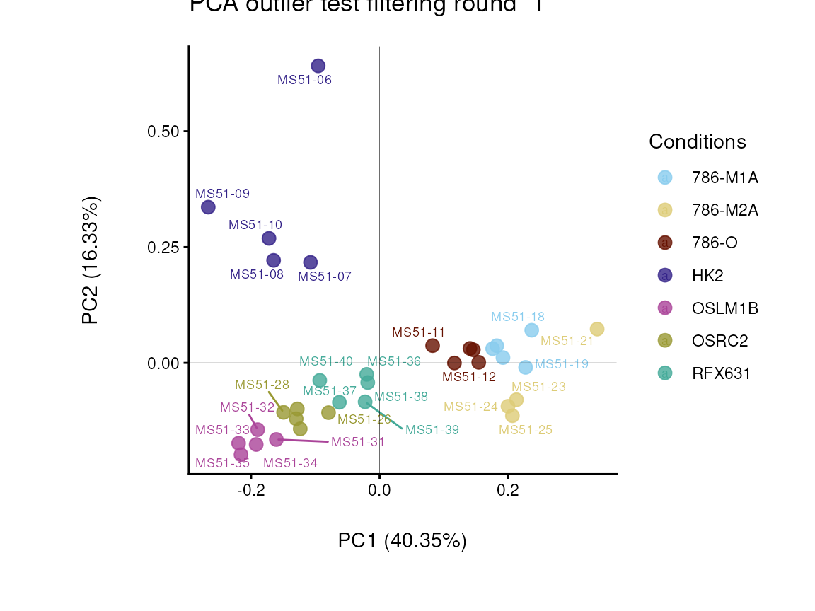
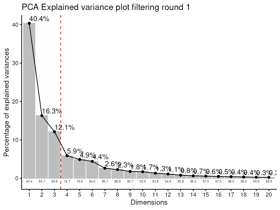
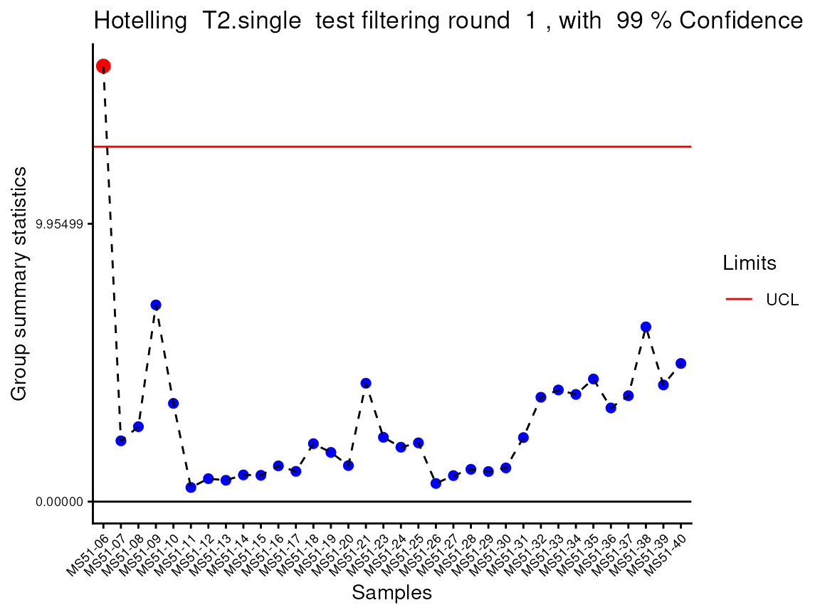
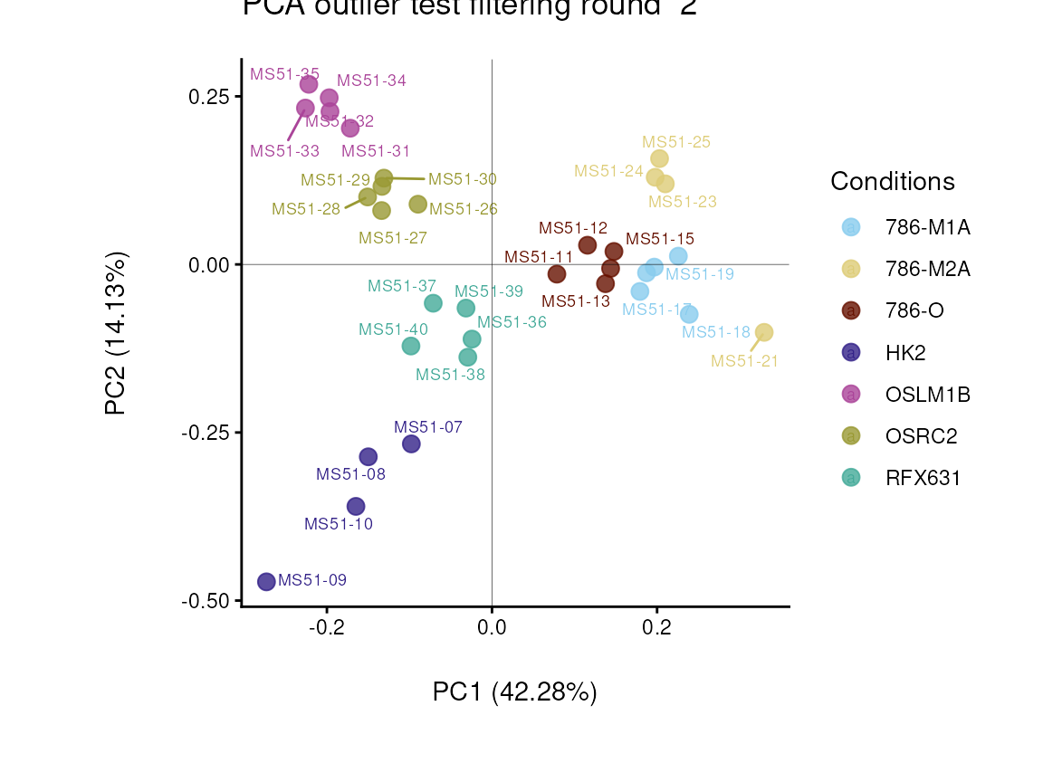
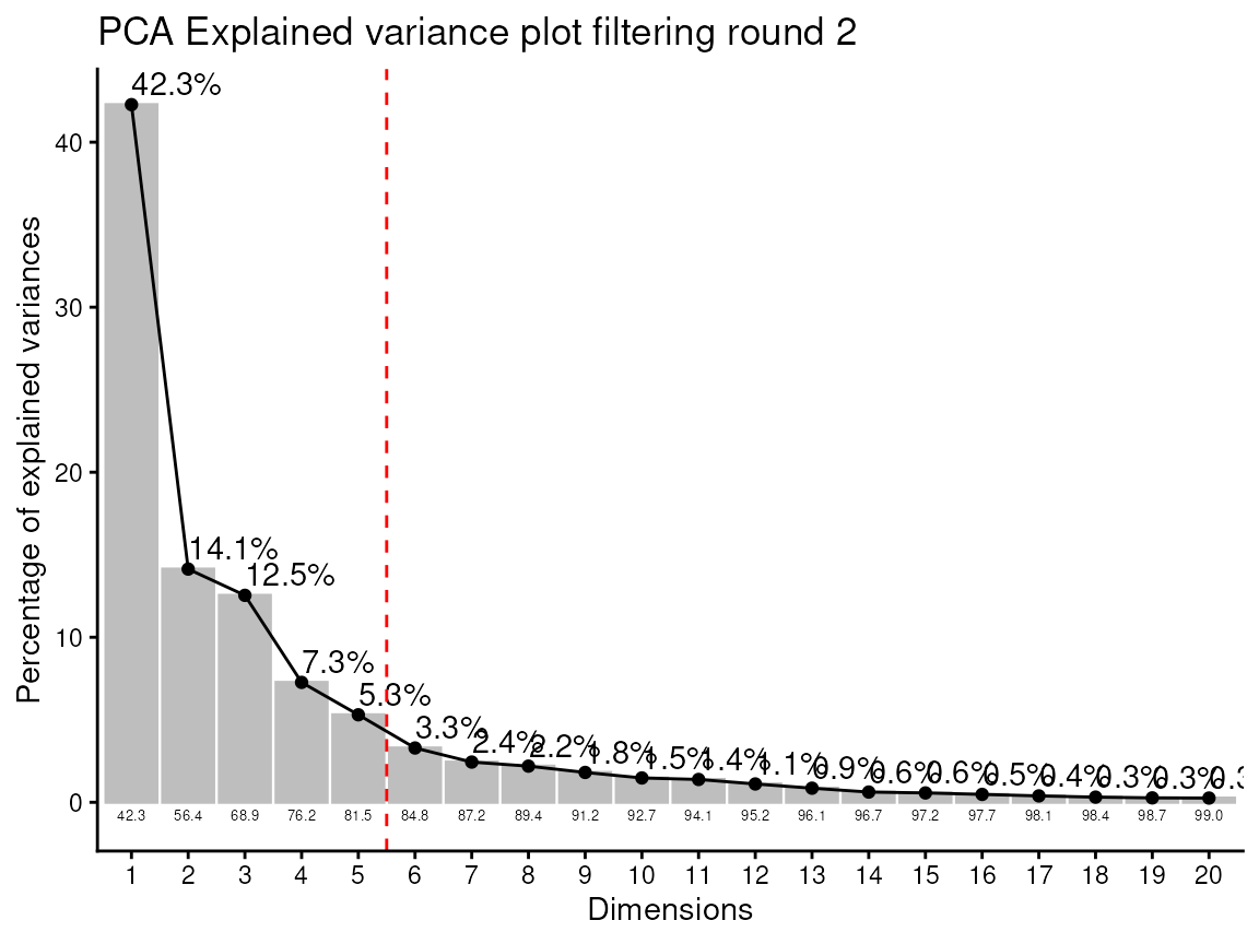
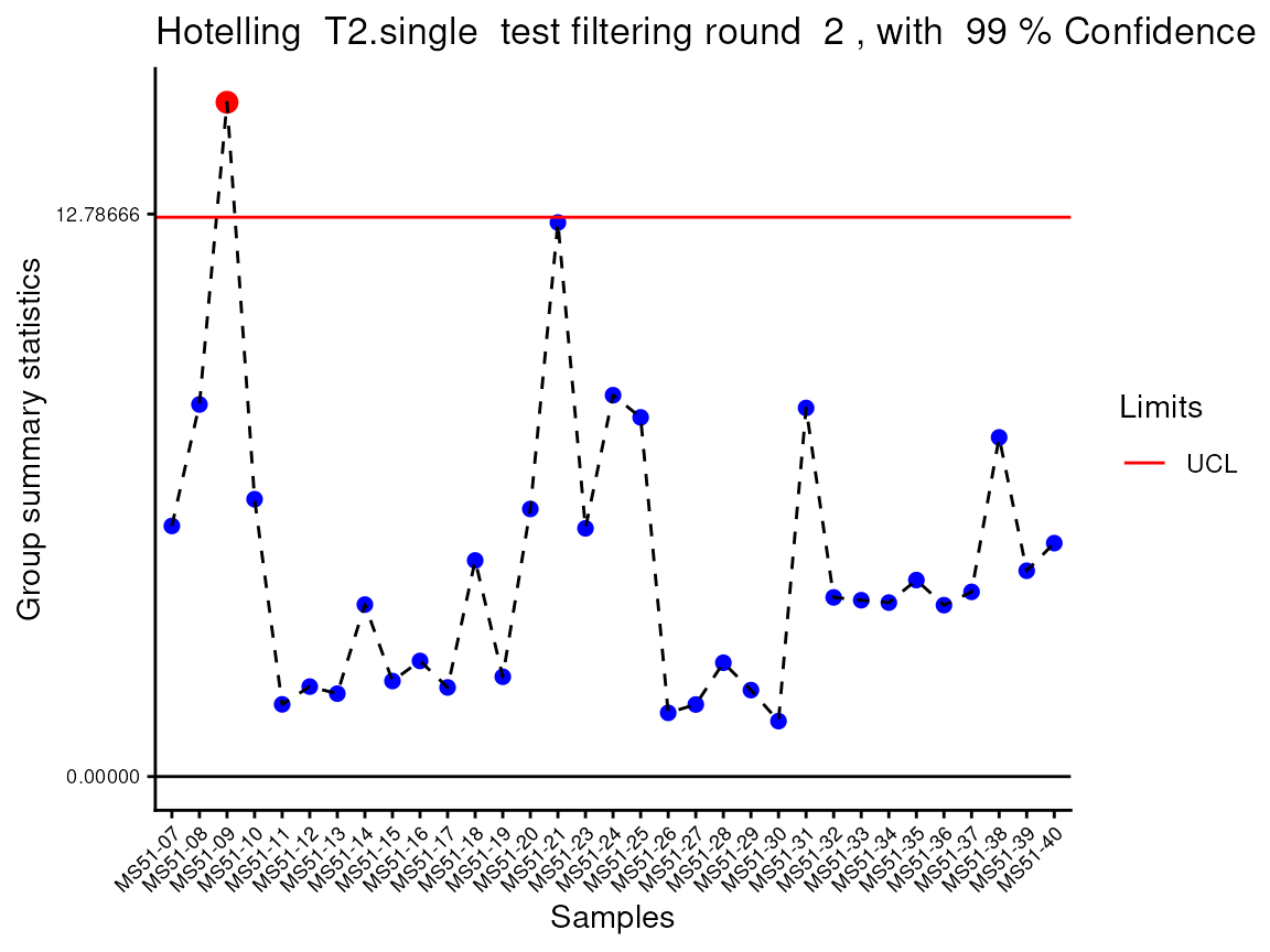
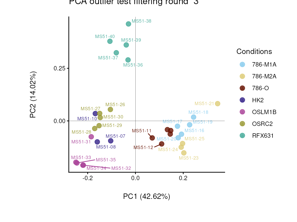
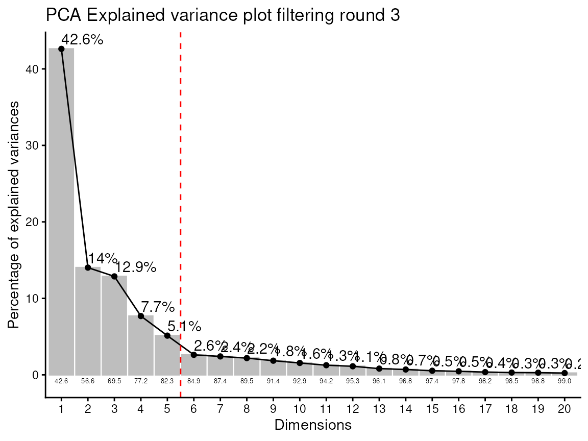
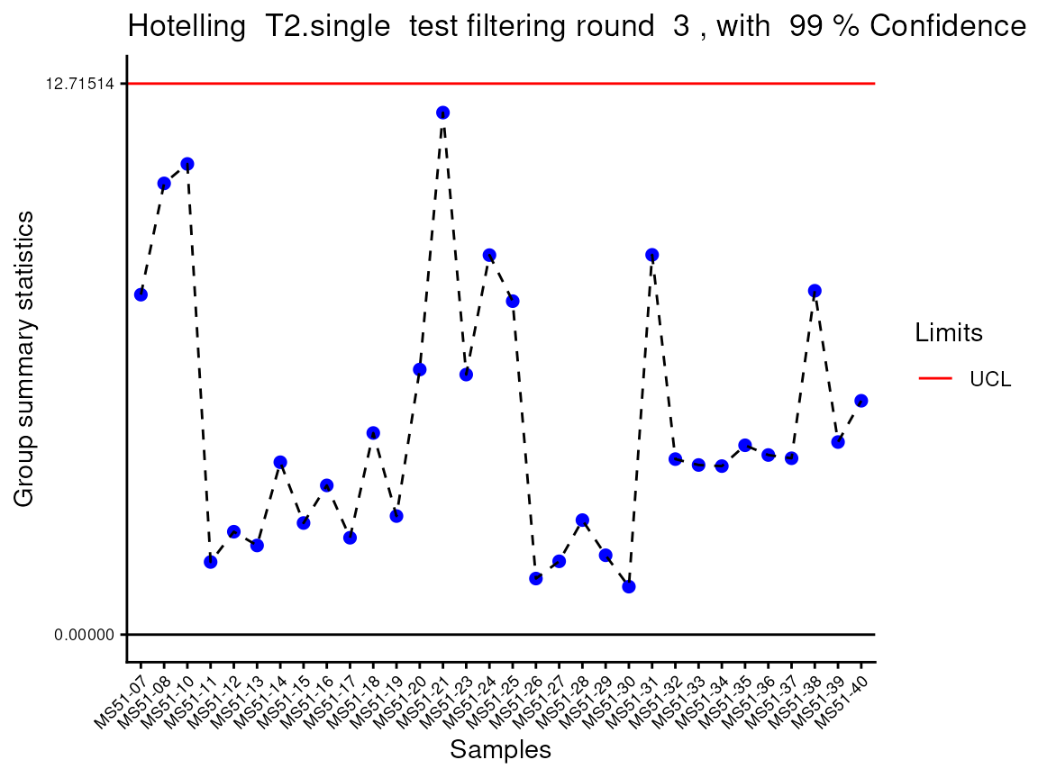
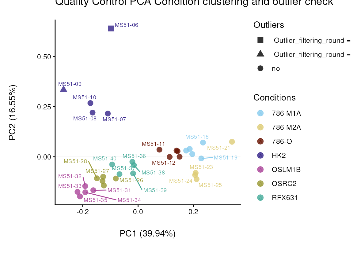
#> Outlier detection: Identification of outlier samples is performed using Hotellin's T2 test to define sample outliers in a mathematical way (Confidence = 0.99 ~ p.val < 0.01) (REF: Hotelling, H. (1931), Annals of Mathematical Statistics. 2 (3), 360-378, doi:https://doi.org/10.1214/aoms/1177732979). hotellins_confidence value selected: 0.99
#> There are possible outlier samples in the data
#> Filtering round  1  Outlier Samples:  MS51-06  
#> Filtering round  2  Outlier Samples:  MS51-09
#> Warning: Removed 5 rows containing non-finite outside the scale range
#> (`stat_boxplot()`).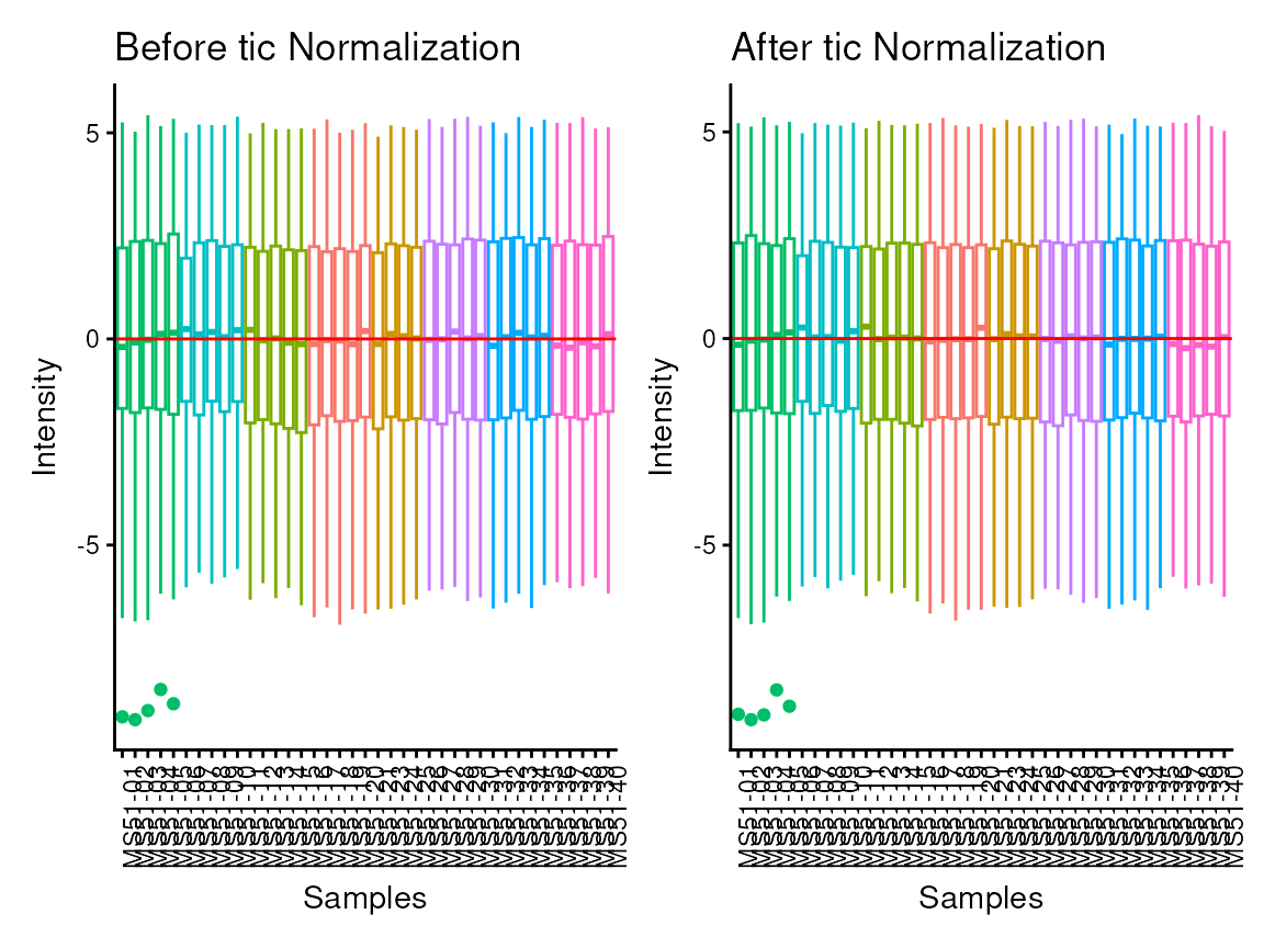

#> Warning: Removed 5 rows containing non-finite outside the scale range
#> (`stat_boxplot()`).
#> Removed 5 rows containing non-finite outside the scale range
#> (`stat_boxplot()`).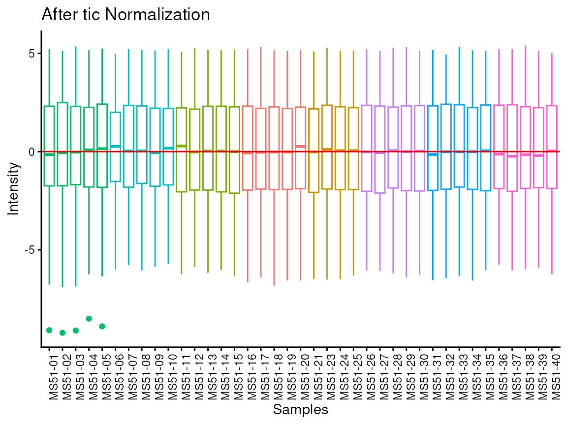

#> Warning: Removed 5 rows containing non-finite outside the scale range
#> (`stat_boxplot()`).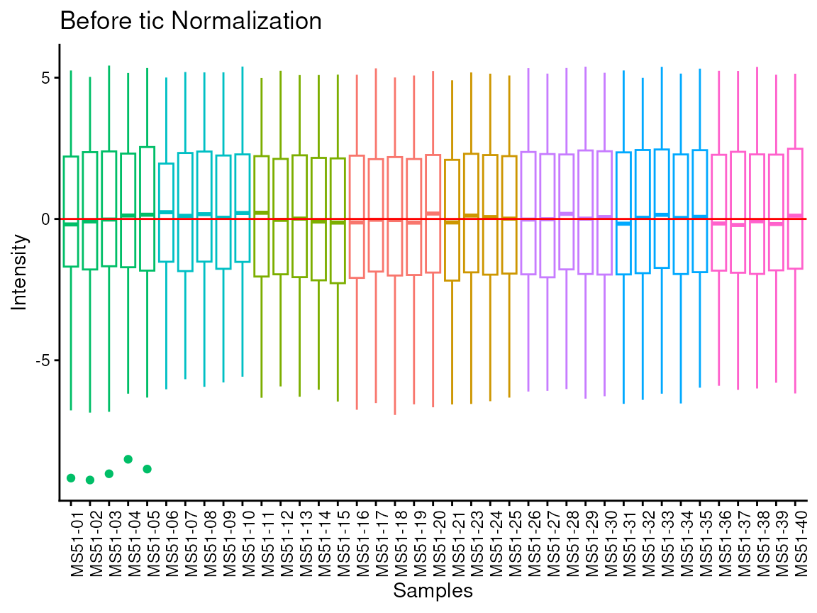

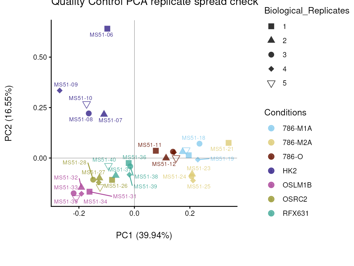
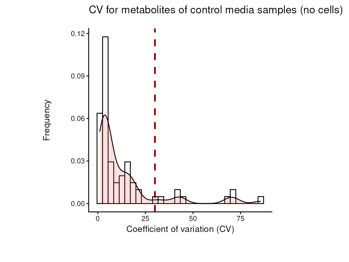
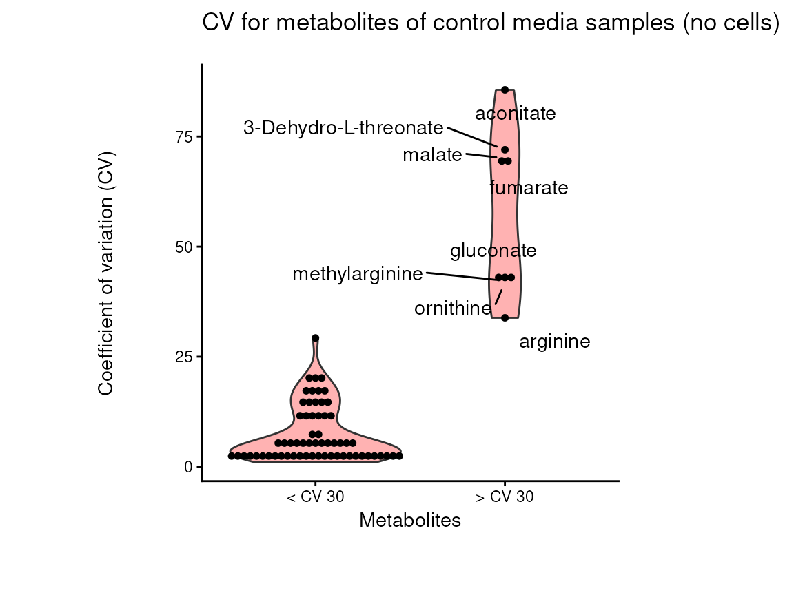
# Now we can have a look at the results table:
Media_Preprocessed <-  PreProcessing_res[["DF"]][["Preprocessing_output"]]

Preview of the pre-processing results, which has an additional column Outlier including the results of Hotelling’s T2.

	Conditions	Biological_Replicates	GrowthFactor	Outliers	valine-d8	hipppuric acid-d5	2-hydroxyglutarate	2-ketoglutarate	3-Dehydro-L-threonate
MS51-06	HK2	1	249.2817	Outlier_filtering_round_1	6622682287	26658050746	5853665424	7527471565	318856944286
MS51-07	HK2	2	249.2817	no	5049281744	30218506574	-868601575	1530912430	28673393701
MS51-08	HK2	3	249.2817	no	-1441406385	-11561761745	1108346025	3684365990	39313101752
MS51-09	HK2	4	249.2817	Outlier_filtering_round_2	2563904070	-10237061776	-189633550	-9097094735	-67782920598
MS51-10	HK2	5	249.2817	no	-6171779428	-8419683053	-50110899	3881816314	-203574855

In the output table you can now see the column “Outliers” and for the Condition HK2 CCM, we can see that based on Hotelling’s T2 test, samples were detected as outliers in the first and second round of filtering.
As part of the processing() function several plots are generated and saved. Additionally, the ggplots are returned into the list to enable further modification using the ggplot syntax. These plots include plots showing the outliers for each filtering round and other QC plots.

As part of the MetaProViz visualization module one can easily further customize the PCA plot and adapt color and shape for the information of interest. You can see more below for the viz_pca() function.
Before we proceed, we will remove the outlier:

Media_Preprocessed <-Media_Preprocessed%>%
subset(!Outliers=="Outlier_filtering_round_1")

In metabolomics, sometimes samples are injected (=measured) several times, which can be termed as analytical replicates. The MetaProViz pre-processing module includes the function replicate_sum(), which will summarize those and save the results.

dma

Differential Metabolite Analysis (dma) between two conditions (e.g. Tumour versus Healthy) usually calculates the Log2FC, p-value, adjusted p-value and t-value. Yet, in a core experiment the normalized metabolite values can be either a negative value, if the metabolite has been consumed from the media, or a positive value, if the metabolite has been released from the cell into the culture media. Since we can not calculate a Log2FC using negative values, we calculate the absolute difference between the mean of Condition 1 versus the mean of Condition 2. The absolute difference is log2 transformed in order to make the values comparable between the different metabolites, resulting in the Log2Dist. The result doesn’t consider whether one product is larger than the other; it only looks at the magnitude of their difference. to reflect the direction of change between the two conditions we multiply with -1 if C1 < C2. By setting the parameter core = TRUE, instead of calculating the Log2FC, the Log2 Distance is calculated.
With the different parameters pval and padj one can choose the statistical tests such as t.test, wilcoxon test, limma, ANOVA, Kruskal-Wallis, etc. (see function reference for more information).
As input one can use the pre-processed data we have generated using the pre-processing module, but here one can of course use any DF including metabolite values, even though we recommend to normalize the data and remove outliers prior to dma. Moreover, we require the metadata_sample including the sample metadata with information which condition a sample corresponds to. Additionally, we enable the user to provide a metadata_feature containing the metadata for the features (metabolites), such as KEGG ID, pathway, retention time, etc.

By defining the numerator and denominator as part of the metadata_info parameter, it is defined which comparisons are performed:
1. one_vs_one (single comparison): numerator=“Condition1”, denominator =“Condition2”
2. all_vs_one (multiple comparison): numerator=NULL, denominator =“Condition”
3. all_vs_all (multiple comparison): numerator=NULL, denominator =NULL (=default)

As input we will use the pre-processed data we have generated using the pre-processing module, but here one can of course use any DF including metabolite values and information about the conditions that should be compared (even though we recommend to normalize the data and remove outliers prior to dma).

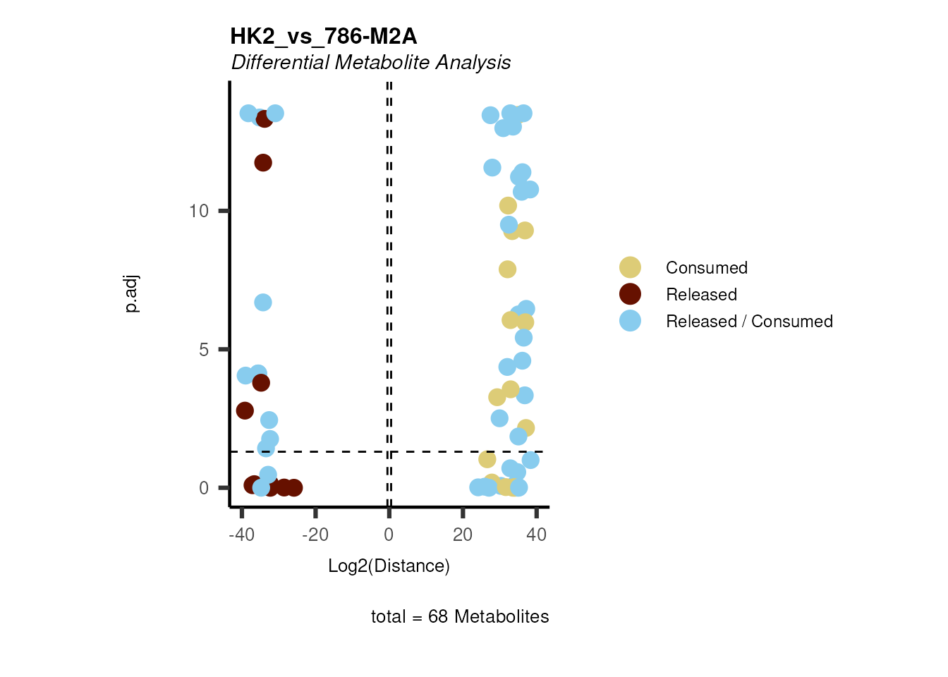
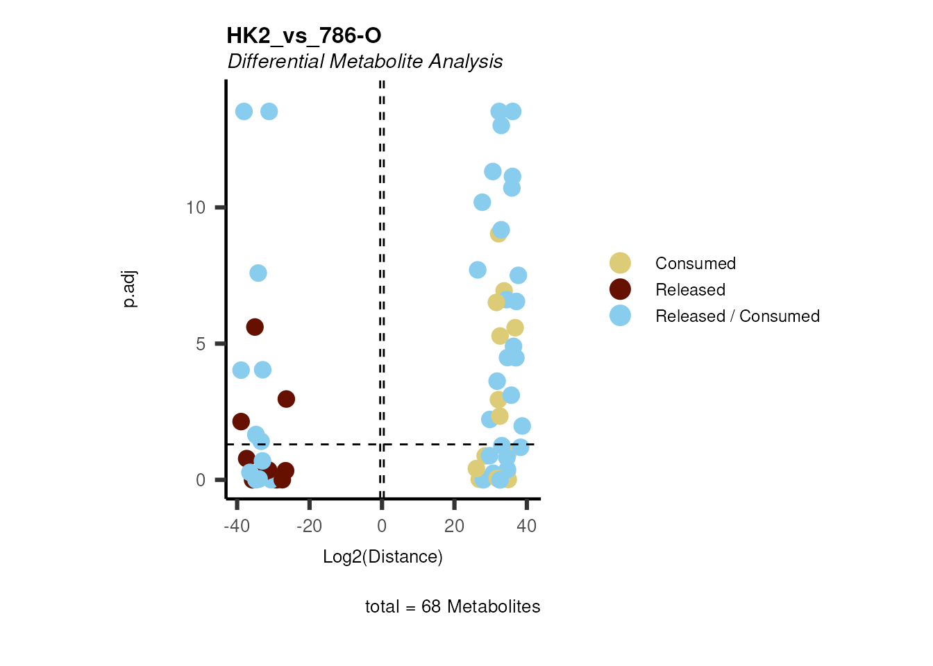
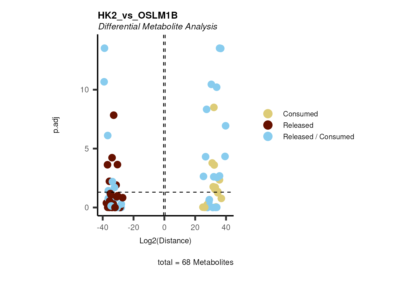
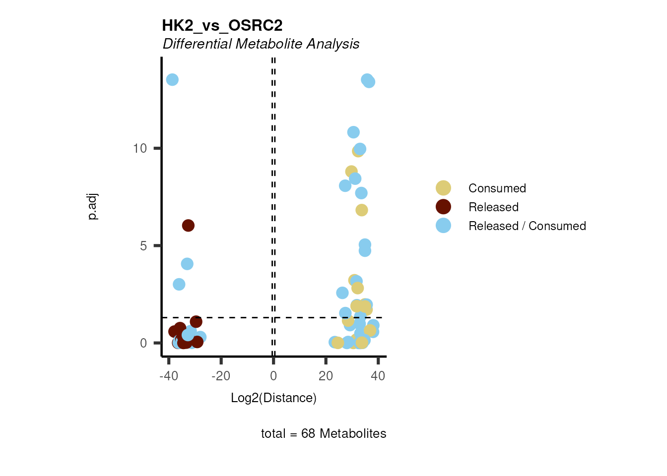
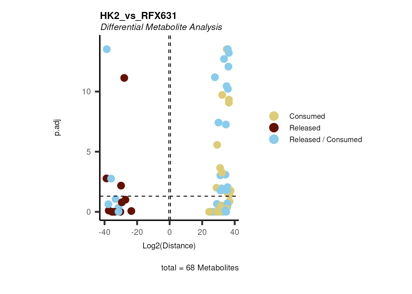
In the example data we have seven different cell lines, healthy (HK2) and cancer (ccRCC: 786-M1A, 786-M2A, 786-O, OSRC2, OSLM1B and RFX631) and hence we can perform multiple different comparisons. The results can be automatically saved and all the results are returned in a list with the different data frames. With print_plot = TRUE and save_plot = "svg" (the defaults), an overview volcano plot is printed and saved.

# Perform multiple comparison All_vs_One using ANOVA:
DMA_Annova <-  dma(data=Media_Preprocessed[,-c(1:6)],
metadata_sample=Media_Preprocessed[,c(1:4)],
metadata_info = c(Conditions="Conditions", Numerator=NULL, Denominator = "HK2"),
pval ="aov",
padj="fdr",
metadata_feature = MappingInfo,
core=TRUE)
#> There are no NA/0 values
#> For 67.65% of metabolites the group variances are equal.
#> We added +1 to the mean value of metabolite(s) , since the mean of the replicate values where 0. This was not due to missing values (NA/0).
#> We added +1 to the mean value of metabolite(s) , since the mean of the replicate values where 0. This was not due to missing values (NA/0).
#> We added +1 to the mean value of metabolite(s) , since the mean of the replicate values where 0. This was not due to missing values (NA/0).
#> We added +1 to the mean value of metabolite(s) , since the mean of the replicate values where 0. This was not due to missing values (NA/0).
#> We added +1 to the mean value of metabolite(s) , since the mean of the replicate values where 0. This was not due to missing values (NA/0).
#> We added +1 to the mean value of metabolite(s) , since the mean of the replicate values where 0. This was not due to missing values (NA/0).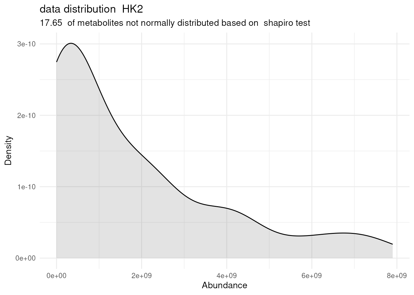

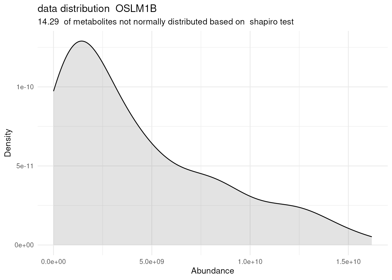
#> `stat_bin()` using `bins = 30`. Pick better value `binwidth`.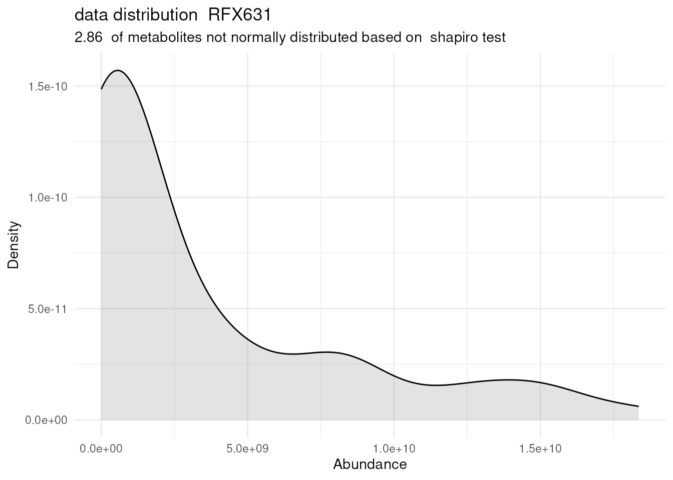

#> `stat_bin()` using `bins = 30`. Pick better value `binwidth`.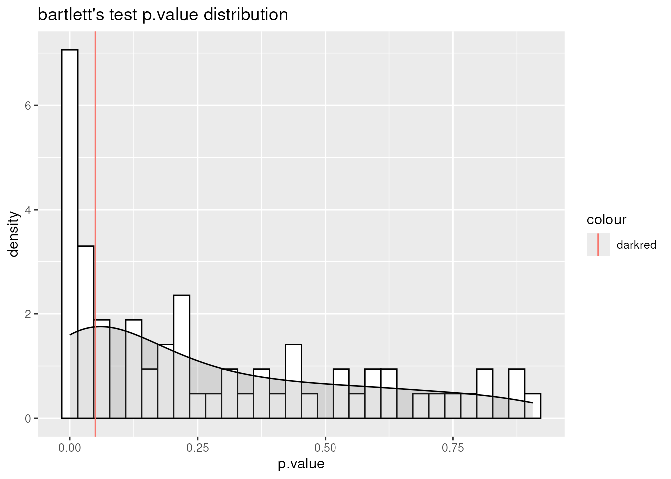

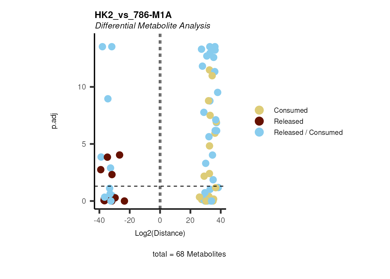
# Inspect the dma results tables:
DMA_HK2_vs_786M1A <- DMA_Annova[["dma"]][["HK2_vs_786-M1A"]]
DMA_HK2_vs_786O <- DMA_Annova[["dma"]][["HK2_vs_786-O"]]
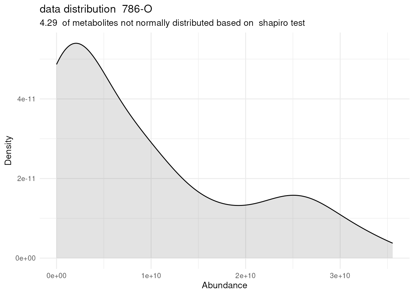
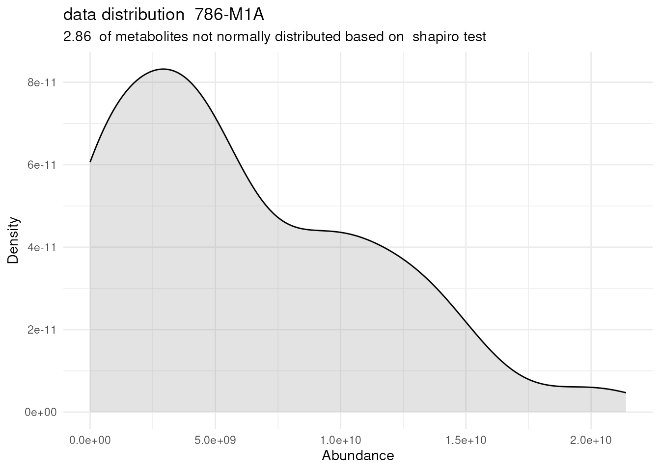
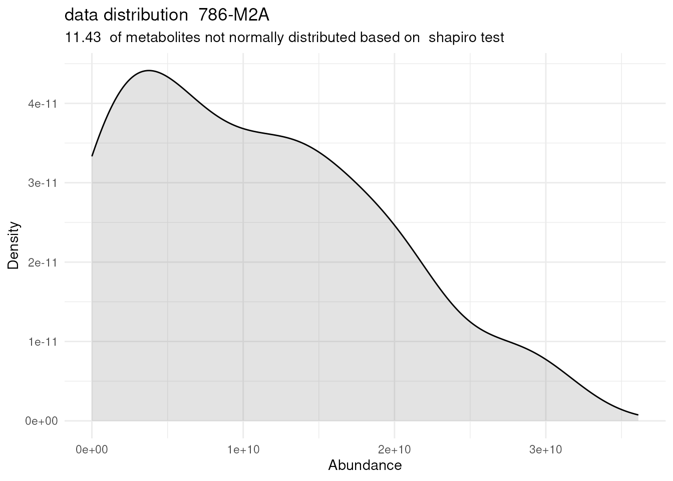
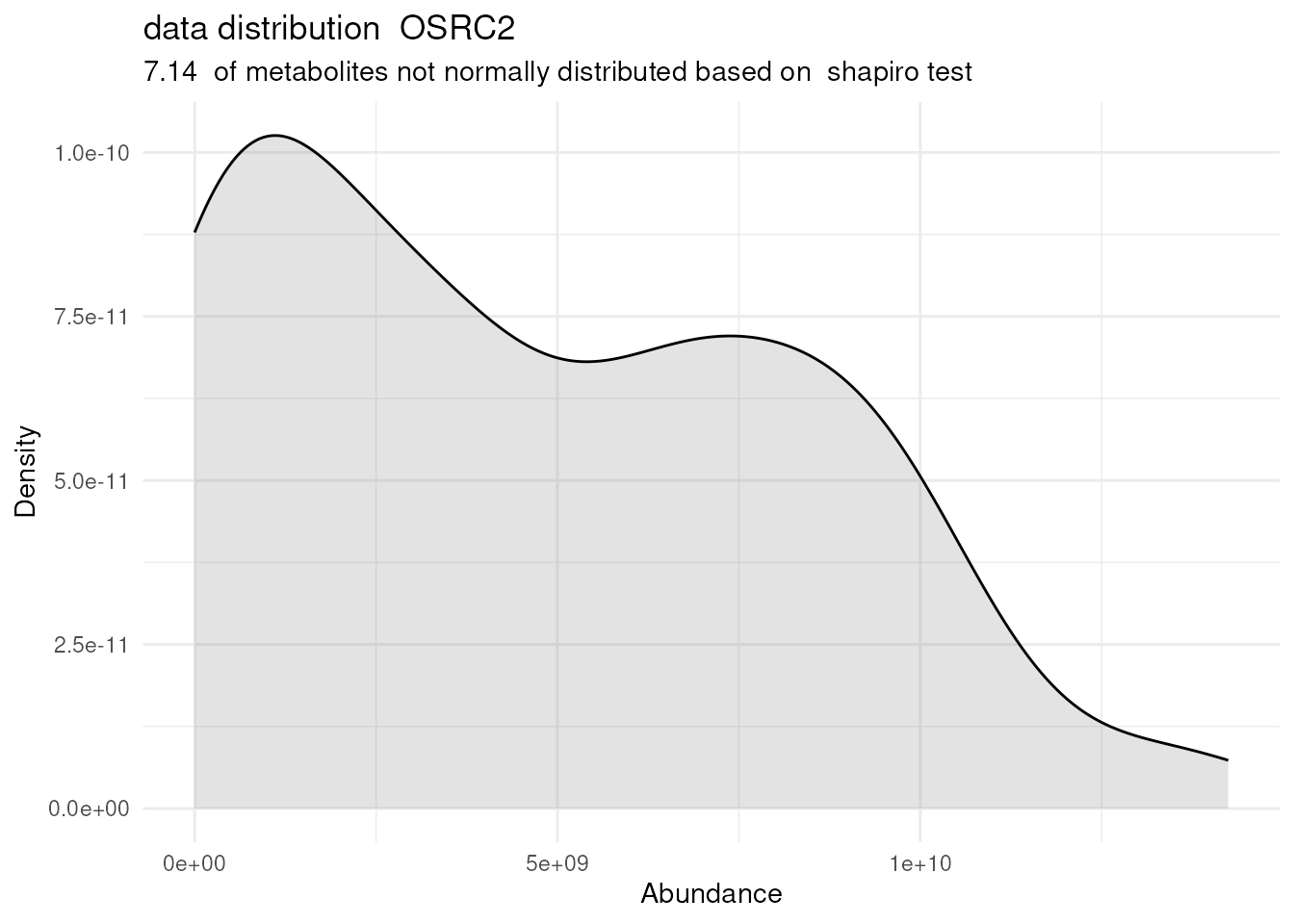
shapiro <- DMA_Annova[["ShapiroTest"]][["DF"]][["Shapiro_result"]]

Preview of the Shapiro results for the different conditions.

Code	Metabolites with normal distribution [%]	Metabolites with not-normal distribution [%]	shapiro p.val(2-hydroxyglutarate)	shapiro p.val(2-ketoglutarate)
HK2	82.35	17.65	0.6833007	0.0446492
786-O	95.71	4.29	0.4938675	0.3823712
786-M1A	97.14	2.86	0.9979050	0.1384610
786-M2A	88.57	11.43	0.5546558	0.5369470
OSRC2	92.86	7.14	0.8899005	0.2007242
OSLM1B	85.71	14.29	0.4643014	0.9022803
RFX631	97.14	2.86	0.9292099	0.0247568

Preview of the dma results for the comparison of 786-M1A versus HK2 cells.

Metabolite	Log2(Distance)	p.adj	t.val	Mean_786-M1A	core_786-M1A	Mean_HK2	core_HK2	core_specific	core	MS51-16	MS51-17	MS51-18	MS51-19	MS51-20	MS51-07	MS51-08	MS51-09	MS51-10	HMDB	KEGG.ID	KEGGCompound	Pathway
aconitate	32.58145	0.0000000	6426780519	-6426780518.51619	Consumed	-9.31322574615479e-07	Consumed	Consumed	Consumed	-5865088200	-6431671420	-6503096254	-6848155621	-6485891098	1186119568	-610503914	-406215498	-169400156	HMDB0000072	C00417	cis-Aconitate	Citrate cycle (TCA cycle)
arginine	-36.63197	0.9411031	-106493120308	106493120307.837	Released	5.7220458984375e-05	Released	Released	Released	216146922501	123584771692	-184582255060	137947177034	239368985373	124885985748	174141953768	-154239029796	-144788909720	HMDB0000517	C00062	L-Arginine	Amino acid metabolism
aspartate	34.35422	0.0000000	21960976607	-21960976606.516	Consumed	-1.72853469848633e-06	Consumed	Consumed	Consumed	-20078854995	-23024873124	-23695204780	-22469858974	-20536091160	1216173971	2386511960	-2796694643	-805991288	HMDB0000191	C00049	L-Aspartate	Amino acid metabolism
betaine	-39.09360	0.0017858	-586606639559	586606639558.529	Released	1.9073486328125e-06	Released	Released	Released	688358341457	490864850765	657311755851	724283773821	372214475898	222640096432	-24221141664	-466988404785	268569450018	HMDB0000043	C00719	Betaine	Not assigned
carbamoyl phosphate	-29.63461	0.5228459	-833502731	833502730.89944	Released	9.23871994018555e-07	Released	Released	Released	544741981	632898115	1989818101	816820279	183235178	200618839	-354809141	549923002	-395732700	HMDB0001096	C00169	Carbamoyl phosphate	Purine metabolism

Using the dma results, we can now use the MetaProViz visualization module and generate further customized Volcano plots viz_volcano(). You can see some examples below.

Additionally to the individual comparison that there is also a summary table created including the individual information about metabolite consumption or release based on the mean measured value:

core_MetaInfo <- DMA_Annova[["Feature_Metadata"]]

Preview of the consumption-release information for each metabolite and cell line.

Metabolite	HMDB	core_786-M1A	core_HK2	core_786-M2A	core_786-O	core_OSLM1B	core_OSRC2	core_RFX631
2-hydroxyglutarate	HMDB0059655	Released	Consumed	Released	Released	Released	Released	Released
acetylcarnitine	HMDB0000201	Consumed	Released	Consumed	Consumed	Consumed	Consumed	Released
acetylcholine	HMDB0000895	Consumed	Released	Consumed	Consumed	Consumed	Consumed	Consumed
acetylornithine	HMDB0003357	Released	Consumed	Released	Released	Released	Released	Released
aconitate	HMDB0000072	Consumed	Consumed	Consumed	Consumed	Consumed	Consumed	Consumed

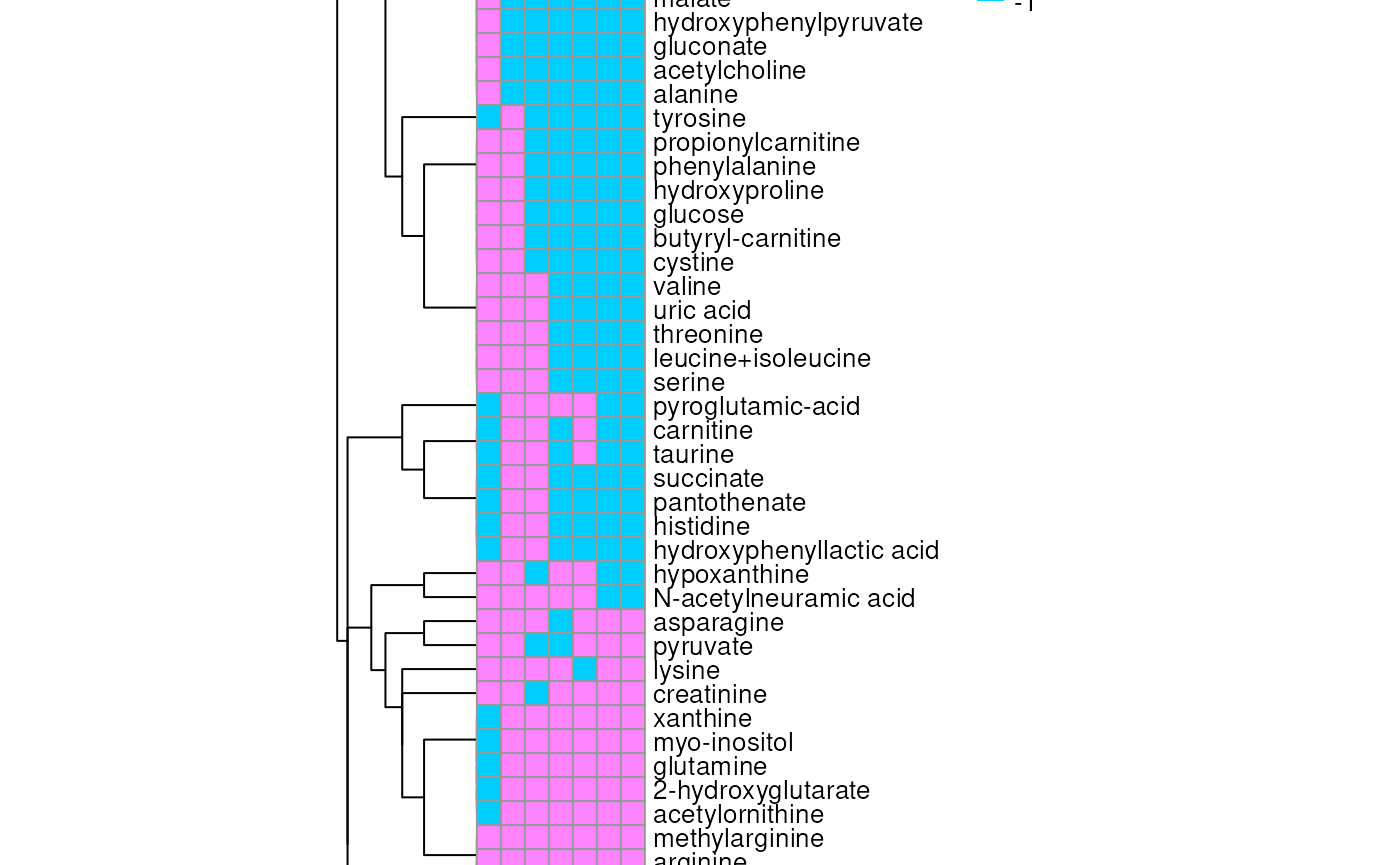
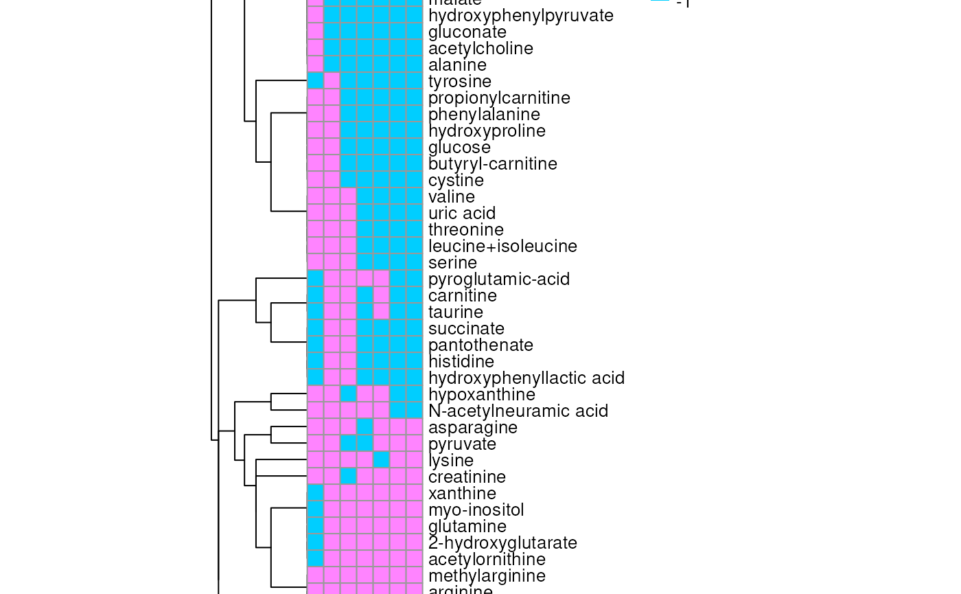
We can also visualize this information by assigning -1 to released, +1 to consumed and 0 for NA:

ORA using the dma results

Over Representation Analysis (ORA) is a pathway enrichment analysis (PEA) method that determines if a set of features (=metabolic pathways) are over-represented in the selection of features (=metabolites) from the data in comparison to all measured features (metabolites) using the Fishers exact test. The selection of metabolites are usually the most altered metabolites in the data, which can be selected by the top and bottom t-values. Given that for core data it is important to consider whether a metabolite was consumed or released, it is sensible to perform ORA on each metabolite cluster.
Of course, there are many other PEA methods such as the well known GSEA. Here we do not aim to provide an extensive tool for different methods to perform pathway enrichment analysis and only focus on ORA since we can apply this to perform standard pathway enrichment as well as pathway enrichment on clusters of metabolites. If you are interested in using different pathway enrichment methods please check out specialized tools such as decoupleR (Badia-I-Mompel et al. 2022).

Here we will use the KEGG pathways (Kanehisa and Goto 2000). Before we can perform ORA on the dma results, we have to ensure that the metabolite names match with the KEGG IDs or KEGG trivial names. In general, the input_pathway requirements are column “term”, “Metabolite” and “Description”, and the data requirements are column “t.val” and column “Metabolite”.

# Since we have performed multiple comparisons (all_vs_HK2), we will run ORA for each of this comparison
DM_ORA_res<- list()

comparisons <- names(DMA_Annova[["dma"]])
for(comparison in comparisons){
    #Ensure that the Metabolite names match with KEGG IDs or KEGG trivial names.
    dma_res <- DMA_Annova[["dma"]][[comparison]]
    dma_res <- dma_res[complete.cases(dma_res),-1]%>%#we remove metabolites that do not have a KEGG ID/KEGG pathway
    tibble::remove_rownames()%>%
    column_to_rownames("KEGGCompound")#We use the KEGG trivial names to match with the KEGG pathways

    #Perform ORA: Here we use
    DM_ORA_res[[comparison]] <- cluster_ora(data=dma_res,
    metadata_info=c(ClusterColumn="core_specific", PathwayTerm= "term", PathwayFeature= "Metabolite"),
    remove_background=FALSE,#we do not have any background
    input_pathway=KEGG_Pathways,
    pathway_name="KEGG",
    min_gssize=3,
    max_gssize=1000)
}

# Lets check how the results look like:
MC_ORA_HK2_vs_786M1A_Consumed <- DM_ORA_res[["HK2_vs_786-M1A"]][["DF"]][["Consumed"]]

Preview of the ORA results for the comparison of 786-M1A versus HK2 cells focusing on pathways enriched in consumed metabolites.

GeneRatio	BgRatio	RichFactor	FoldEnrichment	zScore	pvalue	p.adjust	qvalue	Metabolites_in_pathway	Count	Metabolites_in_Pathway	percentage_of_Pathway_detected
3/13	3/52	1.0000000	4.0000000	3.0606122	0.0129412	0.4464706	0.4464706	L-Aspartate/L-Histidine/Pantothenate	3	32	9.38
3/13	3/52	1.0000000	4.0000000	3.0606122	0.0129412	0.4464706	0.4464706	(9Z)-Octadecenoic acid/Hexadecanoic acid/Octadecanoic acid	3	58	5.17
3/13	15/52	0.2000000	0.8000000	-0.5250483	0.8092578	0.8880214	0.8880214	cis-Aconitate/L-Aspartate/L-Tyrosine	3	144	2.08
4/13	18/52	0.2222222	0.8888889	-0.3333333	0.7455615	0.8880214	0.8880214	L-Aspartate/Glycine/L-Histidine/Taurine	4	130	3.08
2/13	11/52	0.1818182	0.7272727	-0.5824484	0.8354283	0.8880214	0.8880214	L-Aspartate/Succinate	2	27	7.41

MCA

Metabolite Clustering Analysis (MCA) is a module, which includes different functions to enable clustering of metabolites into groups based on logical regulatory rules. This can be particularly useful if one has multiple conditions and aims to find patterns in the data.

mca_core

This metabolite clustering method is based on logical regulatory rules to sort metabolites into metabolite clusters. Here you additionally need intracellular samples corresponding to the core samples.
Here we will define if a feature (= metabolite) is assigned into:
1. “UP”, which means a metabolite is significantly up-regulated in the underlying comparison.
2. “DOWN”, which means a metabolite is significantly down-regulated in the underlying comparison.
3. “No Change”, which means a metabolite does not change significantly in the underlying comparison and/or is not defined as up-regulated/down-regulated based on the Log2FC threshold chosen.

Thereby “No Change” is further subdivided into four states:
1. “Not Detected”, which means a metabolite is not detected in the underlying comparison.
2. “Not Significant”, which means a metabolite is not significant in the underlying comparison.
3. “Significant positive”, which means a metabolite is significant in the underlying comparison and the differential metabolite abundance is positive, yet does not meet the threshold set for “UP” (e.g. Log2FC >1 = “UP” and we have a significant Log2FC=0.8).
4. “Significant negative”, which means a metabolite is significant in the underlying comparison and the differential metabolite abundance is negative, yet does not meet the threshold set for “DOWN”.

Lastly, we also take into account the core direction, meaning if a metabolite was:
1. “Released”, which means is released into the media in both conditions of the underlying comparison.
2. “Consumed”, which means is consumed from the media in both conditions of the underlying comparison.
3. “Released/Consumed”, which means is consumed/released in one condition, whilst the opposite occurs in the second condition of the underlying comparison.
4. “Not Detected”, which means a metabolite is not detected in the underlying comparison.
This definition is done individually for each comparison and will impact in which metabolite cluster a metabolite is sorted into.
Since we have two comparisons (Intracellular and core), we can choose between different Background settings, which defines which features will be considered for the clusters (e.g. you could include only features (= metabolites) that are detected in both comparisons, removing the rest of the features).The background methods method_background are the following from 1.1. - 1.4. from most restrictive to least restrictive:
1.1. Intra&core: Most stringent background setting and will lead to a small number of metabolites.
1.2. core: Focus is on the metabolite abundance of the core.
1.3. Intra: Focus is on the metabolite abundance of intracellular.
1.4. Intra|core: Least stringent background method, since a metabolite will be included in the input if it has been detected on one of the two conditions.

Lastly, we will get clusters of metabolites that are defined by the metabolite change in the two conditions. For example, if Alanine is “UP” based on the thresholds in both comparisons it will be sorted into the cluster “core_UP”. As there are three 6-state6-state4 transitions between the comparisons, the flows are summarised into smaller amount of metabolite clusters using different Regulation Groupings (RG): 1. RG1_All
2. RG2_Significant taking into account genes that are significant (UP, DOWN, significant positive, significant negative)
3. RG3_SignificantChange only takes into account genes that have significant changes (UP, DOWN).

In order to define which group a metabolite is assigned to, we set two different thresholds. For intracellular those are based on the differential metabolite abundance (Log2FC) and the significance (e.g. p.adj). For the core data this is based on the Log2 Distance and the significance (e.g. p.adj). For Log2FC we recommend a threshold of 0.5 or 1, whilst for the Log2 Distance one should check the distance ranges and base the threshold on this.

Regulatory rules:

# Example of all possible flows:
data(mca_core_rules)

MCA_CoRe_Rule <- mca_core_rules

Metabolite Clustering Analysis: core.

Intra	CoRe	Core_Direction	RG1_All	R2_Significant	RG3_Change
DOWN	DOWN	Released	Intra DOWN+ CoRe DOWN_Released	Both_DOWN (Released)	Both_DOWN (Released)
DOWN	Not Detected	Not Detected	Intra DOWN+ CoRe Not Detected	None	None
DOWN	Not Significant	Released	Intra DOWN+ CoRe Not Significant_Released	None	None
DOWN	Significant Negative	Released	Intra DOWN+ CoRe Significant Negative_Released	Both_DOWN (Released)	None
DOWN	Significant Positive	Released	Intra DOWN+ CoRe Significant Positive_Released	Opposite (Released UP)	None
DOWN	UP	Released	Intra DOWN+ CoRe UP_Released	Opposite (Released UP)	Opposite (Released UP)
UP	DOWN	Released	Intra UP+ CoRe DOWN_Released	Opposite (Released DOWN)	Opposite (Released DOWN)
UP	Not Detected	Not Detected	Intra UP+ CoRe Not Detected	None	None
UP	Not Significant	Released	Intra UP+ CoRe Not Significant_Released	None	None
UP	Significant Negative	Released	Intra UP+ CoRe Significant Negative_Released	Opposite (Released UP)	None
UP	Significant Positive	Released	Intra UP+ CoRe Significant Positive_Released	Both_UP (Released)	None
UP	UP	Released	Intra UP+ CoRe UP_Released	Both_UP (Released)	Both_UP (Released)
Not Detected	DOWN	Released	Intra Not Detected+ CoRe DOWN_Released	CoRe_DOWN (Released)	CoRe_DOWN (Released)
Not Detected	Not Detected	Not Detected	Intra Not Detected+ CoRe Not Detected	None	None
Not Detected	Not Significant	Released	Intra Not Detected+ CoRe Not Significant_Released	None	None
Not Detected	Significant Negative	Released	Intra Not Detected+ CoRe Significant Negative_Released	None	None
Not Detected	Significant Positive	Released	Intra Not Detected+ CoRe Significant Positive_Released	None	None
Not Detected	UP	Released	Intra Not Detected+ CoRe UP_Released	CoRe_UP (Released)	CoRe_UP (Released)
Significant Negative	DOWN	Released	Intra Significant Negative+ CoRe DOWN_Released	Both_DOWN (Released)	CoRe_DOWN (Released)
Significant Negative	Not Detected	Not Detected	Intra Significant Negative+ CoRe Not Detected	None	None
Significant Negative	Not Significant	Released	Intra Significant Negative+ CoRe Not Significant_Released	None	None
Significant Negative	Significant Negative	Released	Intra Significant Negative+ CoRe Significant Negative_Released	None	None
Significant Negative	Significant Positive	Released	Intra Significant Negative+ CoRe Significant Positive_Released	None	None
Significant Negative	UP	Released	Intra Significant Negative+ CoRe UP_Released	Opposite (Released UP)	CoRe_UP (Released)
Significant Positive	DOWN	Released	Intra Significant Positive+ CoRe DOWN_Released	Opposite (Released DOWN)	CoRe_DOWN (Released)
Significant Positive	Not Detected	Not Detected	Intra Significant Positive+ CoRe Not Detected	None	None
Significant Positive	Not Significant	Released	Intra Significant Positive+ CoRe Not Significant_Released	None	None
Significant Positive	Significant Negative	Released	Intra Significant Positive+ CoRe Significant Negative_Released	None	None
Significant Positive	Significant Positive	Released	Intra Significant Positive+ CoRe Significant Positive_Released	None	None
Significant Positive	UP	Released	Intra Significant Positive+ CoRe UP_Released	Both_UP (Released)	CoRe_UP (Released)
Not Significant	DOWN	Released	Intra Not Significant+ CoRe DOWN_Released	CoRe_DOWN (Released)	CoRe_DOWN (Released)
Not Significant	Not Detected	Not Detected	Intra Not Significant+ CoRe Not Detected	None	None
Not Significant	Not Significant	Released	Intra Not Significant+ CoRe Not Significant_Released	None	None
Not Significant	Significant Negative	Released	Intra Not Significant+ CoRe Significant Negative_Released	None	None
Not Significant	Significant Positive	Released	Intra Not Significant+ CoRe Significant Positive_Released	None	None
Not Significant	UP	Released	Intra Not Significant+ CoRe UP_Released	CoRe_UP (Released)	CoRe_UP (Released)
DOWN	DOWN	Consumed	Intra DOWN+ CoRe DOWN_Consumed	Both_DOWN (Consumed)	Both_DOWN (Consumed)
DOWN	Not Detected	Not Detected	Intra DOWN+ CoRe Not Detected	None	None
DOWN	Not Significant	Consumed	Intra DOWN+ CoRe Not Significant_Consumed	None	None
DOWN	Significant Negative	Consumed	Intra DOWN+ CoRe Significant Negative_Consumed	Both_DOWN (Consumed)	None
DOWN	Significant Positive	Consumed	Intra DOWN+ CoRe Significant Positive_Consumed	Opposite (Consumed UP)	None
DOWN	UP	Consumed	Intra DOWN+ CoRe UP_Consumed	Opposite (Consumed UP)	Opposite (Consumed UP)
UP	DOWN	Consumed	Intra UP+ CoRe DOWN_Consumed	Opposite (Consumed DOWN)	Opposite (Consumed DOWN)
UP	Not Detected	Not Detected	Intra UP+ CoRe Not Detected	None	None
UP	Not Significant	Consumed	Intra UP+ CoRe Not Significant_Consumed	None	None
UP	Significant Negative	Consumed	Intra UP+ CoRe Significant Negative_Consumed	Opposite (Consumed UP)	None
UP	Significant Positive	Consumed	Intra UP+ CoRe Significant Positive_Consumed	Both_UP (Consumed)	None
UP	UP	Consumed	Intra UP+ CoRe UP_Consumed	Both_UP (Consumed)	Both_UP (Consumed)
Not Detected	DOWN	Consumed	Intra Not Detected+ CoRe DOWN_Consumed	CoRe_DOWN (Consumed)	CoRe_DOWN (Consumed)
Not Detected	Not Detected	Not Detected	Intra Not Detected+ CoRe Not Detected	None	None
Not Detected	Not Significant	Consumed	Intra Not Detected+ CoRe Not Significant_Consumed	None	None
Not Detected	Significant Negative	Consumed	Intra Not Detected+ CoRe Significant Negative_Consumed	None	None
Not Detected	Significant Positive	Consumed	Intra Not Detected+ CoRe Significant Positive_Consumed	None	None
Not Detected	UP	Consumed	Intra Not Detected+ CoRe UP_Consumed	CoRe_UP (Consumed)	CoRe_UP (Consumed)
Significant Negative	DOWN	Consumed	Intra Significant Negative+ CoRe DOWN_Consumed	Both_DOWN (Consumed)	CoRe_DOWN (Consumed)
Significant Negative	Not Detected	Not Detected	Intra Significant Negative+ CoRe Not Detected	None	None
Significant Negative	Not Significant	Consumed	Intra Significant Negative+ CoRe Not Significant_Consumed	None	None
Significant Negative	Significant Negative	Consumed	Intra Significant Negative+ CoRe Significant Negative_Consumed	None	None
Significant Negative	Significant Positive	Consumed	Intra Significant Negative+ CoRe Significant Positive_Consumed	None	None
Significant Negative	UP	Consumed	Intra Significant Negative+ CoRe UP_Consumed	Opposite (Consumed UP)	CoRe_UP (Consumed)
Significant Positive	DOWN	Consumed	Intra Significant Positive+ CoRe DOWN_Consumed	Opposite (Consumed DOWN)	CoRe_DOWN (Consumed)
Significant Positive	Not Detected	Not Detected	Intra Significant Positive+ CoRe Not Detected	None	None
Significant Positive	Not Significant	Consumed	Intra Significant Positive+ CoRe Not Significant_Consumed	None	None
Significant Positive	Significant Negative	Consumed	Intra Significant Positive+ CoRe Significant Negative_Consumed	None	None
Significant Positive	Significant Positive	Consumed	Intra Significant Positive+ CoRe Significant Positive_Consumed	None	None
Significant Positive	UP	Consumed	Intra Significant Positive+ CoRe UP_Consumed	Both_UP (Consumed)	CoRe_UP (Consumed)
Not Significant	DOWN	Consumed	Intra Not Significant+ CoRe DOWN_Consumed	CoRe_DOWN (Consumed)	CoRe_DOWN (Consumed)
Not Significant	Not Detected	Not Detected	Intra Not Significant+ CoRe Not Detected	None	None
Not Significant	Not Significant	Consumed	Intra Not Significant+ CoRe Not Significant_Consumed	None	None
Not Significant	Significant Negative	Consumed	Intra Not Significant+ CoRe Significant Negative_Consumed	None	None
Not Significant	Significant Positive	Consumed	Intra Not Significant+ CoRe Significant Positive_Consumed	None	None
Not Significant	UP	Consumed	Intra Not Significant+ CoRe UP_Consumed	CoRe_UP (Consumed)	CoRe_UP (Consumed)
DOWN	DOWN	Released/Consumed	Intra DOWN + CoRe DOWN_Released/Consumed	Both_DOWN (Released/Consumed)	Both_DOWN (Released/Consumed)
DOWN	Not Detected	Not Detected	Intra DOWN + CoRe Not Detected	None	None
DOWN	Not Significant	Released/Consumed	Intra DOWN + CoRe Not Significant_Released/Consumed	None	None
DOWN	Significant Negative	Released/Consumed	Intra DOWN + CoRe Significant Negative_Released/Consumed	Both_DOWN (Released/Consumed)	None
DOWN	Significant Positive	Released/Consumed	Intra DOWN + CoRe Significant Positive_Released/Consumed	Opposite (Released/Consumed UP)	None
DOWN	UP	Released/Consumed	Intra DOWN + CoRe UP_Released/Consumed	Opposite (Released/Consumed UP)	Opposite (Released/Consumed UP)
UP	DOWN	Released/Consumed	Intra UP + CoRe DOWN_Released/Consumed	Opposite (Released/Consumed DOWN)	Opposite (Released/Consumed DOWN)
UP	Not Detected	Not Detected	Intra UP + CoRe Not Detected	None	None
UP	Not Significant	Released/Consumed	Intra UP + CoRe Not Significant_Released/Consumed	None	None
UP	Significant Negative	Released/Consumed	Intra UP + CoRe Significant Negative_Released/Consumed	Opposite (Released/Consumed UP)	None
UP	Significant Positive	Released/Consumed	Intra UP + CoRe Significant Positive_Released/Consumed	Both_UP (Released/Consumed)	None
UP	UP	Released/Consumed	Intra UP + CoRe UP_Released/Consumed	Both_UP (Released/Consumed)	Both_UP (Released/Consumed)
Not Detected	DOWN	Released/Consumed	Intra Not Detected + CoRe DOWN_Released/Consumed	CoRe_DOWN (Released/Consumed)	CoRe_DOWN (Released/Consumed)
Not Detected	Not Detected	Not Detected	Intra Not Detected + CoRe Not Detected	None	None
Not Detected	Not Significant	Released/Consumed	Intra Not Detected + CoRe Not Significant_Released/Consumed	None	None
Not Detected	Significant Negative	Released/Consumed	Intra Not Detected + CoRe Significant Negative_Released/Consumed	None	None
Not Detected	Significant Positive	Released/Consumed	Intra Not Detected + CoRe Significant Positive_Released/Consumed	None	None
Not Detected	UP	Released/Consumed	Intra Not Detected + CoRe UP_Released/Consumed	CoRe_UP (Released/Consumed)	CoRe_UP (Released/Consumed)
Significant Negative	DOWN	Released/Consumed	Intra Significant Negative + CoRe DOWN_Released/Consumed	Both_DOWN (Released/Consumed)	CoRe_DOWN (Released/Consumed)
Significant Negative	Not Detected	Not Detected	Intra Significant Negative + CoRe Not Detected	None	None
Significant Negative	Not Significant	Released/Consumed	Intra Significant Negative + CoRe Not Significant_Released/Consumed	None	None
Significant Negative	Significant Negative	Released/Consumed	Intra Significant Negative + CoRe Significant Negative_Released/Consumed	None	None
Significant Negative	Significant Positive	Released/Consumed	Intra Significant Negative + CoRe Significant Positive_Released/Consumed	None	None
Significant Negative	UP	Released/Consumed	Intra Significant Negative + CoRe UP_Released/Consumed	Opposite (Released/Consumed UP)	CoRe_UP (Released/Consumed)
Significant Positive	DOWN	Released/Consumed	Intra Significant Positive + CoRe DOWN_Released/Consumed	Opposite (Released/Consumed DOWN)	CoRe_DOWN (Released/Consumed)
Significant Positive	Not Detected	Not Detected	Intra Significant Positive + CoRe Not Detected	None	None
Significant Positive	Not Significant	Released/Consumed	Intra Significant Positive + CoRe Not Significant_Released/Consumed	None	None
Significant Positive	Significant Negative	Released/Consumed	Intra Significant Positive + CoRe Significant Negative_Released/Consumed	None	None
Significant Positive	Significant Positive	Released/Consumed	Intra Significant Positive + CoRe Significant Positive_Released/Consumed	None	None
Significant Positive	UP	Released/Consumed	Intra Significant Positive + CoRe UP_Released/Consumed	Both_UP (Released/Consumed)	CoRe_UP (Released/Consumed)
Not Significant	DOWN	Released/Consumed	Intra Not Significant + CoRe DOWN_Released/Consumed	CoRe_DOWN (Released/Consumed)	CoRe_DOWN (Released/Consumed)
Not Significant	Not Detected	Not Detected	Intra Not Significant + CoRe Not Detected	None	None
Not Significant	Not Significant	Released/Consumed	Intra Not Significant + CoRe Not Significant_Released/Consumed	None	None
Not Significant	Significant Negative	Released/Consumed	Intra Not Significant + CoRe Significant Negative_Released/Consumed	None	None
Not Significant	Significant Positive	Released/Consumed	Intra Not Significant + CoRe Significant Positive_Released/Consumed	None	None
Not Significant	UP	Released/Consumed	Intra Not Significant + CoRe UP_Released/Consumed	CoRe_UP (Released/Consumed)	CoRe_UP (Released/Consumed)

Now we can load the corresponding pre-processed intracellular example data for the comparison of 786M-1A versus HK2 (For the detailed pre-processing please see the vignette “Standard Metabolomics”).

# Load the Pre-processed intracellular data:
data(intracell_dma)

Intra_DMA_HK2_vs_786M1A <- intracell_dma%>%
as.data.frame()

# Perform metabolite clustering:
MCA_core_res <- mca_core(data_intra =Intra_DMA_HK2_vs_786M1A,
data_core = DMA_HK2_vs_786M1A,
metadata_info_intra=c(ValueCol="Log2FC",StatCol="p.adj", cutoff_stat= 0.05, ValueCutoff=0.8),
metadata_info_core=c(DirectionCol="core", ValueCol="Log2(Distance)",StatCol="p.adj", cutoff_stat= 0.05, ValueCutoff=28),
feature= "Metabolite",
method_background="Intra&core",
path=NULL)

# Lets check how the results look like:
MCA_res <- MCA_core_res[["MCA_core_Results"]]
Clustersummary <- MCA_core_res[["MCA_core_summary"]]

mca_core for the comparison of 786-M1A versus HK2 cells in intracellular and core samples.

Metabolite	Intra_DF_Cutoff	Intra_DF_Cutoff_Specific.x	core_DF_Detected	core_DF_Cutoff	core_DF_Cutoff_Specific	BG_method	RG1_All	RG2_Significant	RG3_Change
adenosine	No Change	Not Significant	FALSE	No Change	Not Detected	FALSE	Background = FALSE	Background = FALSE	Background = FALSE
ADP	No Change	Not Significant	FALSE	No Change	Not Detected	FALSE	Background = FALSE	Background = FALSE	Background = FALSE
betaine	DOWN	DOWN	TRUE	DOWN	DOWN	TRUE	Intra DOWN + core DOWN_Released	Both_DOWN (Released)	Both_DOWN (Released)
creatine	No Change	Significant Positive	TRUE	DOWN	DOWN	TRUE	NA	NA	NA

mca_core summary of number of metabolites per cluster.

Regulation Grouping	SiRCle cluster Name	Number of Features
RG3_Change	Both_DOWN (Released)	2
RG3_Change	core_UP (Consumed)	4
RG3_Change	core_DOWN (Released)	1

Now we can also create Bargraphs of the clusters to visualize the results. Here we create two summary bargraphs for the Regulation Grouping RG2 and RG3:

#> Warning: No shared levels found between `names(values)` of the manual scale and the
#> data's fill values.
#> No shared levels found between `names(values)` of the manual scale and the
#> data's fill values.
#> No shared levels found between `names(values)` of the manual scale and the
#> data's fill values.
#> No shared levels found between `names(values)` of the manual scale and the
#> data's fill values.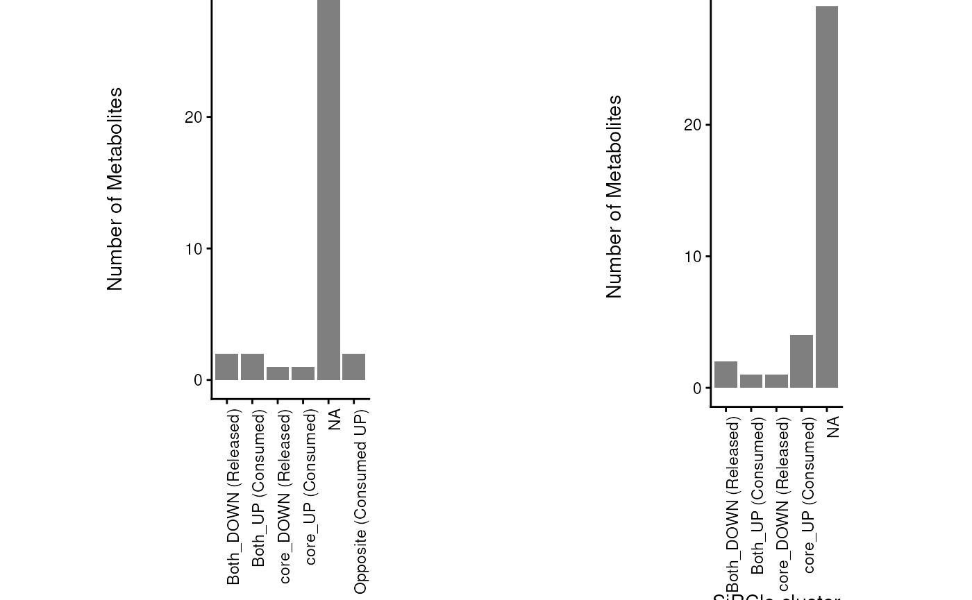

MetaLinksDB metabolite-receptor and metabolite-transporter sets

The MetaLinks database is a manually curated database of metabolite-receptor and metabolite-transporter sets that can be used to study the connection of metabolites and receptors or transporters (Farr et al. 2024).
To remove potential false positives and decrease the number of putative metabolite-receptor interactions, we filter the MetalinksDB resource to metabolites that are annotated as present in the kidney, blood, or urine in HMDB and known to be extracellular.

# Selection as described in ST2 of Farr_Dimitrov2024:
MetaLinksDB <- metsigdb_metalinks(cell_location =c("Extracellular"),
tissue_location = c("Kidney", "All Tissues"),
biospecimen_location = c("Blood",  "Urine"))

# Here we add a UniquePair column combining hmdb-protein connection, removing duplications originating from different PK resources
MetaLinksDB_Select <- MetaLinksDB %>%
tidyr::unite("UniquePair", c("hmdb", "gene_symbol"), sep = "_", remove=FALSE)%>%
distinct(UniquePair, .keep_all = TRUE)

Now we can use this information to understand if the metabolites that are consumed in the 786-M1A cells and Released in the HK2 cells are connected to specific receptors or transporters and are in the bioRCM cluster “Both_DOWN (Released/Consumed)

#> The following metabolites are not connected to any receptor or transporter in the MetalinksDB:
#> The following metabolites are connected to at least one receptor or transporter in the MetalinksDB: betaine, asparagine

The same filtered MetaLinksDB table can be visualized directly as a metabolite-protein network with viz_pk_network(). Via metadata_info we tell the function which columns hold the metabolite IDs and names in our data and the IDs and proteins in MetalinksDB. The metabolite name column is recommended, but only the ID columns are required. We additionally colour the edges by the interaction type, use the line type for the mode of regulation and draw the edges in the direction provided by metsigdb_metalinks().

MetaLinks_Features <- MCA_res %>%
    dplyr::filter(RG2_Significant == "Both_DOWN (Released)") %>%
    dplyr::filter(!is.na(core_DF_HMDB)) %>%
    dplyr::distinct(Metabolite, core_DF_HMDB)

MetaLinks_Network <- viz_pk_network(
    feature_metadata = MetaLinks_Features,
    input_pk = MetaLinksDB_Select,
    metadata_info = c(
        InputID = "core_DF_HMDB",
        InputLabel = "Metabolite",
        PriorID = "hmdb",
        PriorTerm = "gene_symbol",
        EdgeColor = "interaction",
        EdgeLinetype = "mode_of_regulation",
        EdgeDirection = "direction"
    ),
    save_plot = NULL,
    print_plot = TRUE,
    label_mode = "all",
    seed = 123
)

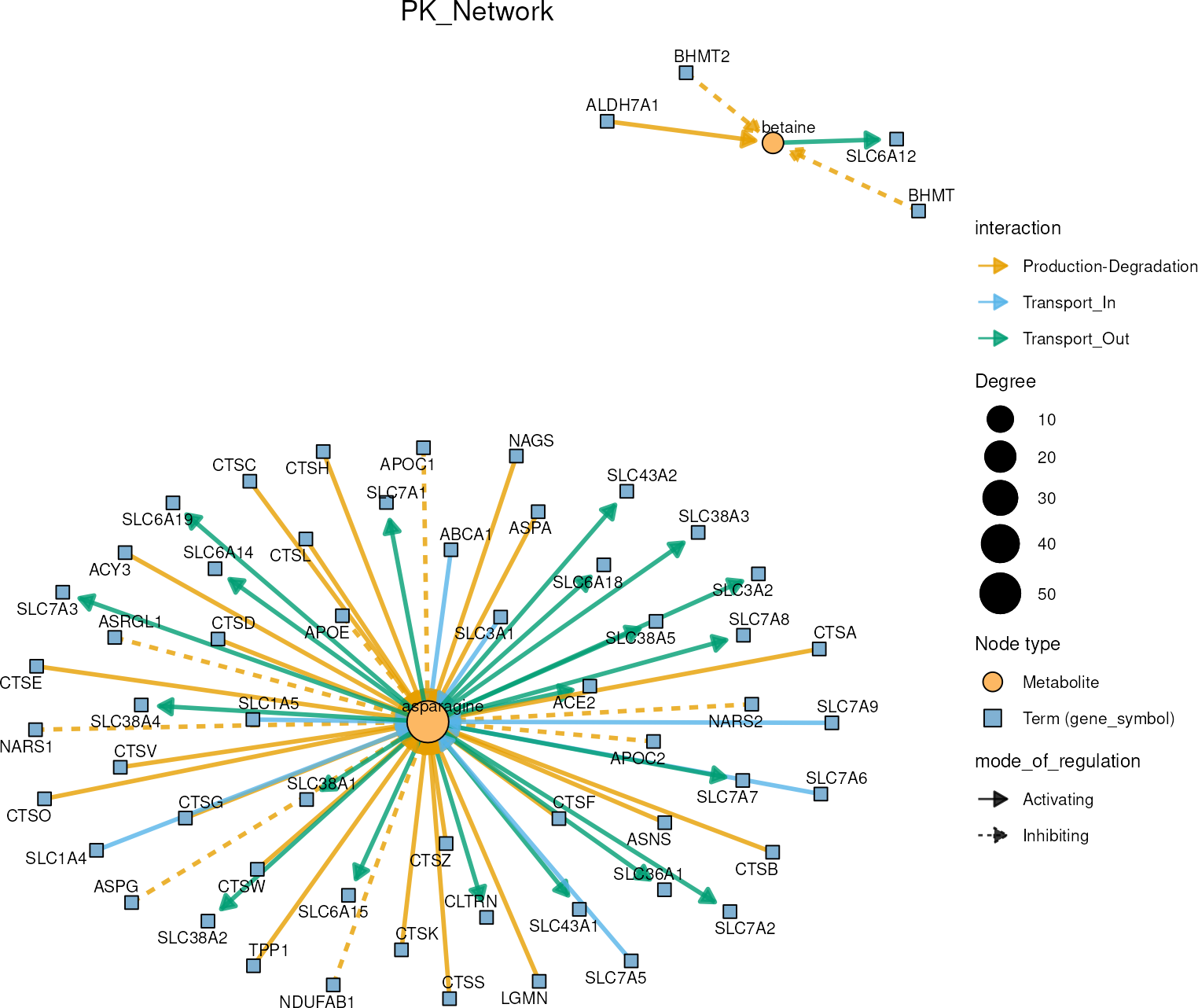
From this visualization, we gain insight into cellular mechanisms for metabolites of interest. In our case, we can see “betaine” and “asparagine” interactions with transporters, receptors and other metabolic enzymes which are curated in MetalinksDB.
This is only one example of how prior knowledge networks help to investigate specific results. In the Prior Knowledge Networks vignette we show many more, e.g. which transporters the changed metabolites share, which metabolites drive the enriched pathways and in which cancers the metabolites have been reported before.

ORA on each metabolite cluster

As explained in detail above, Over Representation Analysis (ORA) is a pathway enrichment analysis (PEA) method. As ORA is based on the Fishers exact test it is perfect to test if a set of features (=metabolic pathways) are over-represented in the selection of features (= clusters of metabolites) from the data in comparison to all measured features (all metabolites). In detail, cluster_ora() will perform ORA on each of the metabolite clusters using all metabolites as the background.

Pathway input for cluster_ora().

	HMDB	KEGG.ID	KEGGCompound	Pathway
N-acetylaspartate	HMDB0000812	C01042	N-Acetyl-L-aspartate	Alanine, aspartate and glutamate metabolism
argininosuccinate	HMDB0000052	C03406	N-(L-Arginino)succinate	Alanine, aspartate and glutamate metabolism
N-acetylaspartylglutamate	HMDB0001067	C12270	N-Acetylaspartylglutamate	Alanine, aspartate and glutamate metabolism
tyrosine	HMDB0000158	C00082	L-Tyrosine	Amino acid metabolism
asparagine	HMDB0000168	C00152	L-Asparagine	Amino acid metabolism
glutamate	HMDB0000148	C00025	L-Glutamate	Amino acid metabolism

MC_ORA_result<- cluster_ora(data=MCA_core_res[["MCA_core_Results"]]%>%column_to_rownames("Metabolite"),
metadata_info=c(ClusterColumn="RG2_Significant",
                                                        BackgroundColumn="BG_method",
                                                        PathwayTerm= "Pathway", #This is the column name including the pathways names
                                                        PathwayFeature= "Metabolite"),
                                                        remove_background=TRUE,
                                                        input_pathway=MappingInfo%>%rownames_to_column("Metabolite"),
                                                        pathway_name="KEGG",
                                                        min_gssize=3,
                                                        max_gssize=1000 ,
                                                        save_table= "csv")

cluster_ora() results for the RG2_Significant cluster Both_DOWN (Consumed).

Here we see that the pathways have a low amount of genes included that were also part of the cluster and the pathways are not significant. This is due to multiple factors, first we only start with a small number of metabolites with KEGG IDs and secondly we only included metabolites if they were detected in both, intracellular and core samples (parameter method_background="Intra&core"). Hence, by for example setting parameter method_background="Intra|core", we will obtain larger metabolite clusters.

Run MetaProViz Visualisation

The big advantages of the MetaProViz visualization module is its flexible and easy usage, which we will showcase below and that the figures are saved in a publication ready style and format. For instance, the x- and y-axis size will always be adjusted for the amount of samples or features (=metabolites) plotted, or in the case of Volcano plot and PCA plot the axis size is fixed and not affected by figure legends or title. In this way, there is no need for many adjustments and the figures can just be dropped into the presentation or paper and are all in the same style.

All the viz_*() functions are constructed in the same way. Indeed, with the parameter metadata_info the user can pass a named vector with information about the metadata column that should be used to customize the plot by colour, shape or creating individual plots, which will all be showcased for the different plot types. Via the parameters metadata_sample and metadata_feature the user can pass the metadata DF for the samples and/or the features (=metabolites), depending on the plot type.

In each of those plots, the user can label color and/or shape based on additional information (e.g. Pathway information, Cluster information or other other demographics like gender). Moreover, we also enable to plot individual plots where applicable based on those MetaData (e.g. one plot for each metabolic pathway).
For this we need a metadata table including information about our samples that could be relevant to e.g. color code:

MetaData_Sample <- Media_Preprocessed[,c(1:2)]%>%
mutate(Status = case_when(Conditions=="HK2" ~ 'Healthy',
TRUE ~ 'Cancer'))

Metadata table including additional information about our Samples.

	Conditions	Biological_Replicates	Status
MS51-07	HK2	2	Healthy
MS51-08	HK2	3	Healthy
MS51-09	HK2	4	Healthy
MS51-10	HK2	5	Healthy
MS51-11	786-O	1	Cancer
MS51-12	786-O	2	Cancer
MS51-13	786-O	3	Cancer
MS51-14	786-O	4	Cancer
MS51-15	786-O	5	Cancer
MS51-16	786-M1A	1	Cancer
MS51-17	786-M1A	2	Cancer
MS51-18	786-M1A	3	Cancer
MS51-19	786-M1A	4	Cancer
MS51-20	786-M1A	5	Cancer
MS51-21	786-M2A	1	Cancer
MS51-23	786-M2A	2	Cancer
MS51-24	786-M2A	3	Cancer
MS51-25	786-M2A	4	Cancer
MS51-26	OSRC2	1	Cancer
MS51-27	OSRC2	2	Cancer
MS51-28	OSRC2	3	Cancer
MS51-29	OSRC2	4	Cancer
MS51-30	OSRC2	5	Cancer
MS51-31	OSLM1B	1	Cancer
MS51-32	OSLM1B	2	Cancer
MS51-33	OSLM1B	3	Cancer
MS51-34	OSLM1B	4	Cancer
MS51-35	OSLM1B	5	Cancer
MS51-36	RFX631	1	Cancer
MS51-37	RFX631	2	Cancer
MS51-38	RFX631	3	Cancer
MS51-39	RFX631	4	Cancer
MS51-40	RFX631	5	Cancer

Moreover, we can use MetaData for our features (=Metabolites), which we loaded with the MappingInfo and we can also add the information on which cluster a metabolite was assigned to in the mca_core() analysis above:

MetaData_Metab <- merge(
    MappingInfo %>% rownames_to_column("Metabolite"),
    MCA_res %>% dplyr::select(Metabolite, dplyr::starts_with("RG")),
    by = "Metabolite",
    all.x = TRUE
) %>%
    column_to_rownames("Metabolite")

Metadata table including additional information about the Metabolites.

HMDB	KEGG.ID	KEGGCompound	Pathway	RG1_All	RG2_Significant	RG3_Change
HMDB0000208	C00026	2-Oxoglutarate	Citrate cycle (TCA cycle)	NA	NA	NA
HMDB0060180	C00197	3-Phospho-D-glycerate	Glycolysis / Gluconeogenesis	Background = FALSE	Background = FALSE	Background = FALSE
HMDB0003464	C01035	4-Guanidinobutanoate	Arginine and proline metabolism	Background = FALSE	Background = FALSE	Background = FALSE
HMDB0000052	C03406	N-(L-Arginino)succinate	Alanine, aspartate and glutamate metabolism	Background = FALSE	Background = FALSE	Background = FALSE
HMDB0000168	C00152	L-Asparagine	Amino acid metabolism	Intra DOWN + core DOWN_Released	Both_DOWN (Released)	Both_DOWN (Released)
HMDB0000191	C00049	L-Aspartate	Amino acid metabolism	Intra Significant Positive + core UP_Consumed	Both_UP (Consumed)	core_UP (Consumed)

Noteworthy, here we can also use the KEGG pathways we used for the pathway analysis.

PCA plots

Principal component analysis (PCA) is a dimensionality reduction method that reduces all the measured features (=metabolites) of one sample into a few features in the different principal components, whereby each principal component can explain a certain percentage of the variance between the different samples. Hence, this enables interpretation of sample clustering based on the measured features (=metabolites).
As mentioned above, PCA plots can be quite useful for quality control, but of course it offers us many more opportunities, which will be showcased here.

As input, we need a DF that contains the samples as rownames and the features (=metabolites) as column names:

Input_PCA <- Media_Preprocessed[,-c(1:4)] #remove columns that include Metadata such as cell type,...

Input data for viz_pca(), with samples as rownames and metabolites as column names.

	valine-d8	hipppuric acid-d5	2-hydroxyglutarate	2-ketoglutarate	3-Dehydro-L-threonate	acetylcarnitine	acetylcholine
MS51-07	5049281744	30218506574	-868601575	1530912430	28673393701	-67547592848	-496576017
MS51-08	-1441406385	-11561761745	1108346025	3684365990	39313101752	-234677799645	-124297109
MS51-09	2563904070	-10237061776	-189633550	-9097094735	-67782920598	218513442831	526295913
MS51-10	-6171779428	-8419683053	-50110899	3881816314	-203574855	83711949661	94577213
MS51-11	27378617230	123649127347	4311754839	23286535748	-16721754062	-434945308541	-183109349
MS51-12	31998154622	99965859879	808357705	19381509727	-16349278172	-583665678018	-998475065

Now lets check out the standard plot:

viz_pca(data=Input_PCA)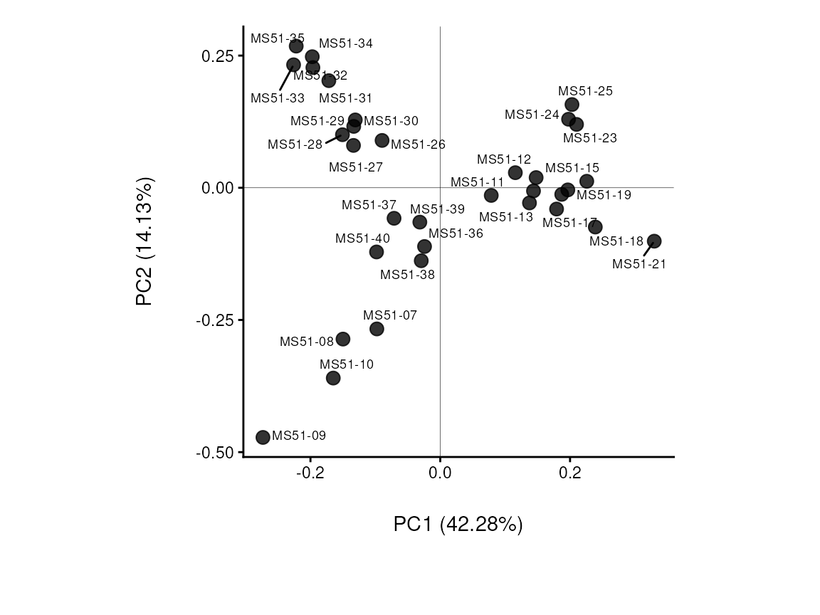

Standard Settings.

Next, we can interactively choose shape and color using the additional information of interest from our Metadata. Especially for complex data, such as patient data, it can be valuable to use different demographics (e.g. age, gender, medication,…) for this. First lets check if we have any batch effect by colour coding for the biological replicates, which would be the case if the replicates cluster together.

viz_pca(metadata_info= c(color="Biological_Replicates"),
metadata_sample = MetaData_Sample ,
data=Input_PCA,
plot_name = "Batch Effect")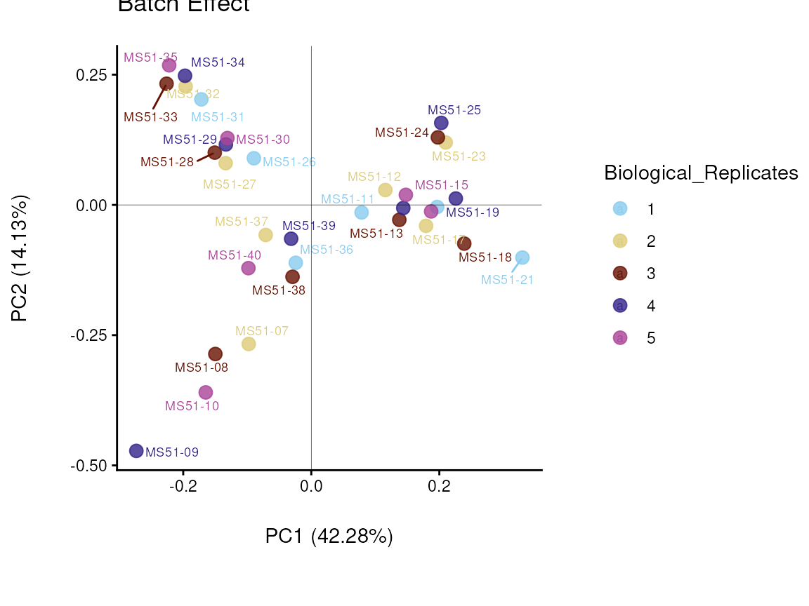

Do we have a batch effect?

Given the biological replicates are numeric, we can also set color_scale to continuous:

viz_pca(metadata_info= c(color="Biological_Replicates"),
metadata_sample = MetaData_Sample ,
data=Input_PCA,
scale_color = "continuous",
plot_name = "Batch Effect (continuous color scale)")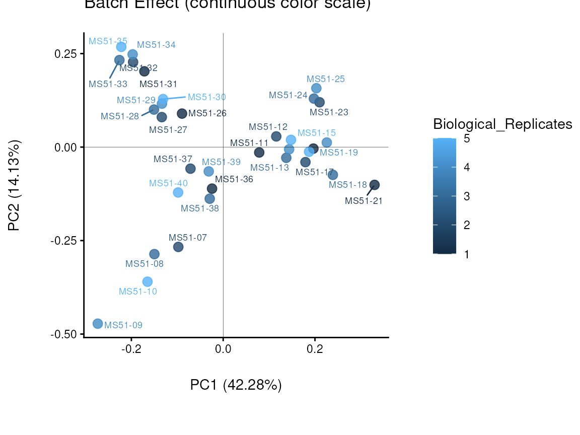

Do we have a batch effect?

Next, we can colour code for condition and use the biological replicates in the shape parameter:

viz_pca(metadata_info= c(color="Conditions", shape="Biological_Replicates"),
metadata_sample = MetaData_Sample ,
data=Input_PCA,
plot_name = "Sample Conditions")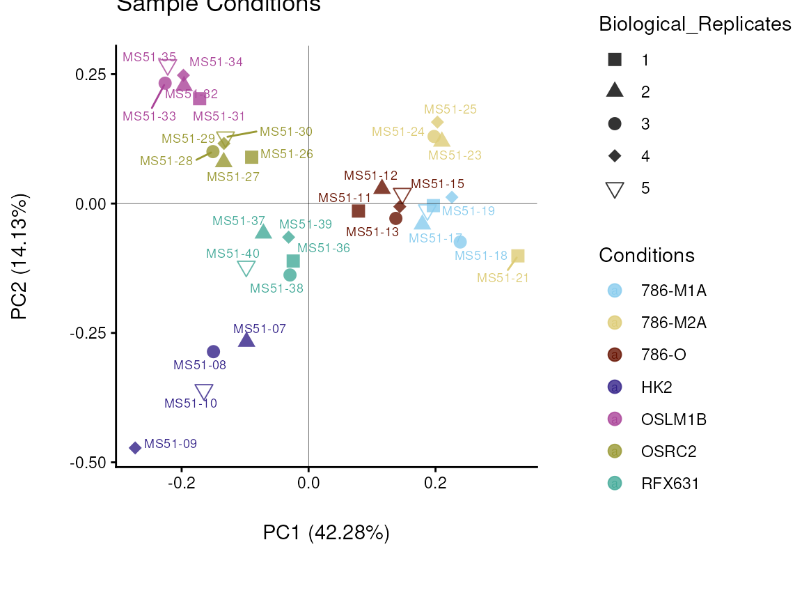

Do the samples cluster for the conditions?

The different cell lines we have are either control or cancerous, so we can display this too.

viz_pca(metadata_info=  c(color="Status"),
metadata_sample = MetaData_Sample ,
data=Input_PCA,
plot_name = "Sample Status")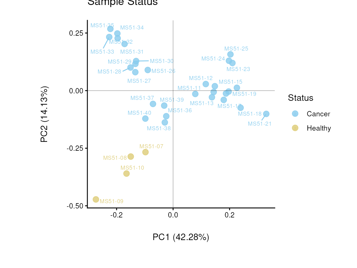

Do the samples cluster for the Cell status?

Heatmaps

Clustered heatmaps can be useful to understand the patterns in the data, which will be showcased on different examples.
As input, we need a DF that contains the samples as rownames and the features (=metabolites) as column names:

Input_Heatmap <-   Media_Preprocessed[,-c(1:6)] #remove columns that include Metadata such as cell type,...

# Add consumption-release information of each cell type:
MetaData_Metab <- DMA_Annova[["Feature_Metadata"]]%>%
column_to_rownames("Metabolite")

Input for viz_heatmap(), with samples as rownames and metabolites as column names.

	2-hydroxyglutarate	2-ketoglutarate	3-Dehydro-L-threonate	acetylcarnitine	acetylcholine
MS51-07	-868601575	1530912430	28673393701	-67547592848	-496576017
MS51-08	1108346025	3684365990	39313101752	-234677799645	-124297109
MS51-09	-189633550	-9097094735	-67782920598	218513442831	526295913
MS51-10	-50110899	3881816314	-203574855	83711949661	94577213
MS51-11	4311754839	23286535748	-16721754062	-434945308541	-183109349
MS51-12	808357705	19381509727	-16349278172	-583665678018	-998475065

Now we can generate an overview heatmap. Since we plot all metabolites the metabolite names are not plotted since this would get too crowded (You can enforce this by changing the parameter enforce_featurenames = TRUE).

viz_heatmap(data = Input_Heatmap,
plot_name = "Overview")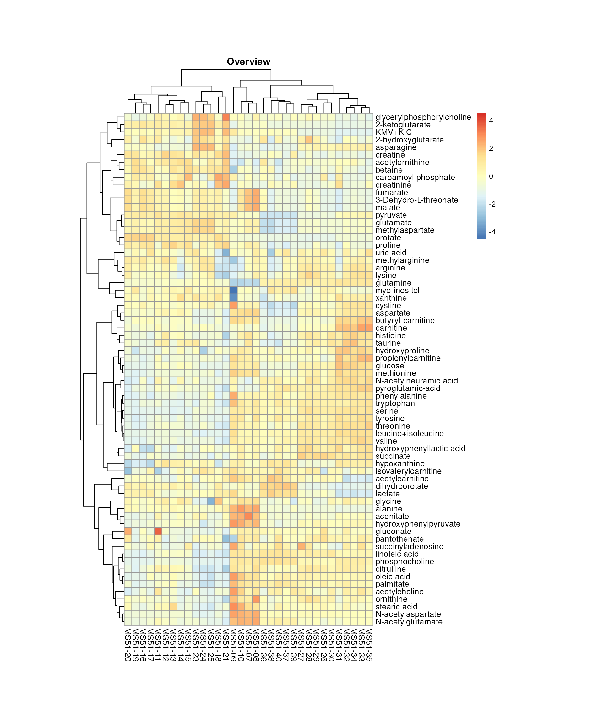

Overview heatmap.

Here we can add as many sample metadata information as needed at the same time:

viz_heatmap(data = Input_Heatmap,
metadata_sample = MetaData_Sample,
metadata_info = c(color_Sample = list("Conditions","Biological_Replicates", "Status")),
plot_name = "Colour Samples")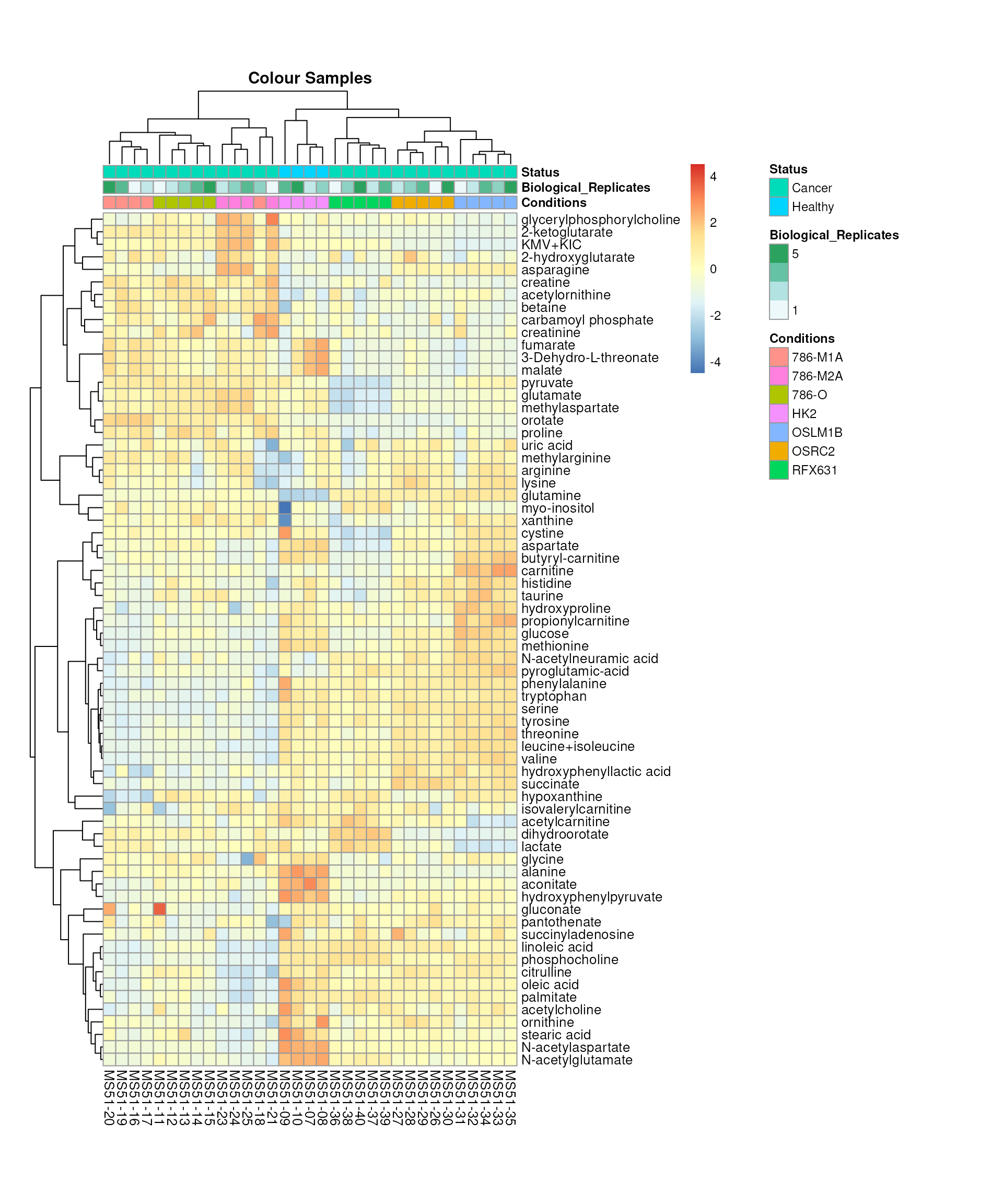

Colour for sample metadata.

Moreover, we can also add metabolite metadata information:

viz_heatmap(data = Input_Heatmap,
metadata_sample = MetaData_Sample,
metadata_info = c(color_Metab = list("Pathway",  "core_786-M1A", "core_HK2", "core_786-M2A", "core_786-O", "core_OSLM1B", "core_OSRC2", "core_RFX631"),
                                        color_Sample = list("Conditions","Biological_Replicates", "Status")),
                                        metadata_feature =  MetaData_Metab,
                                        plot_name = "Colour Metabolites")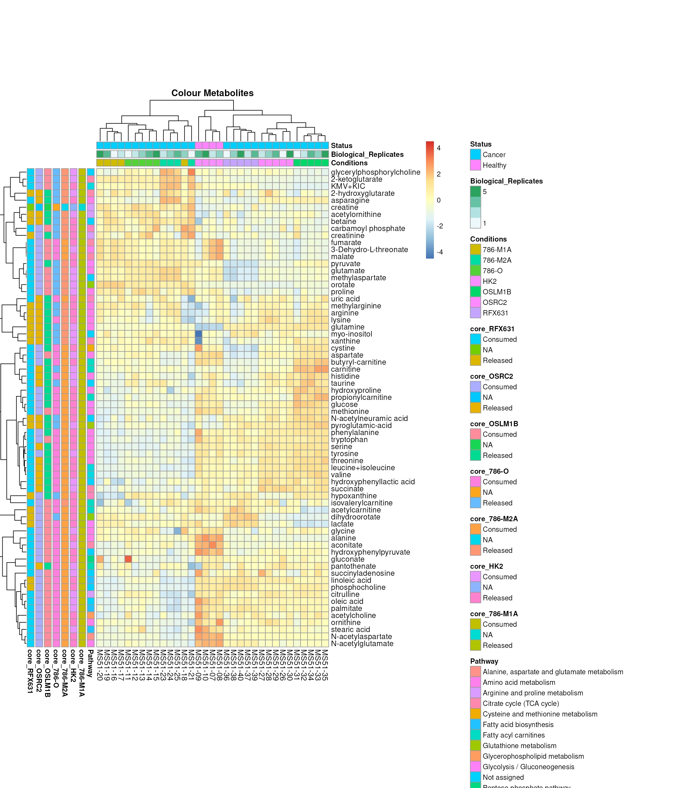

Colour for metabolite metadata.

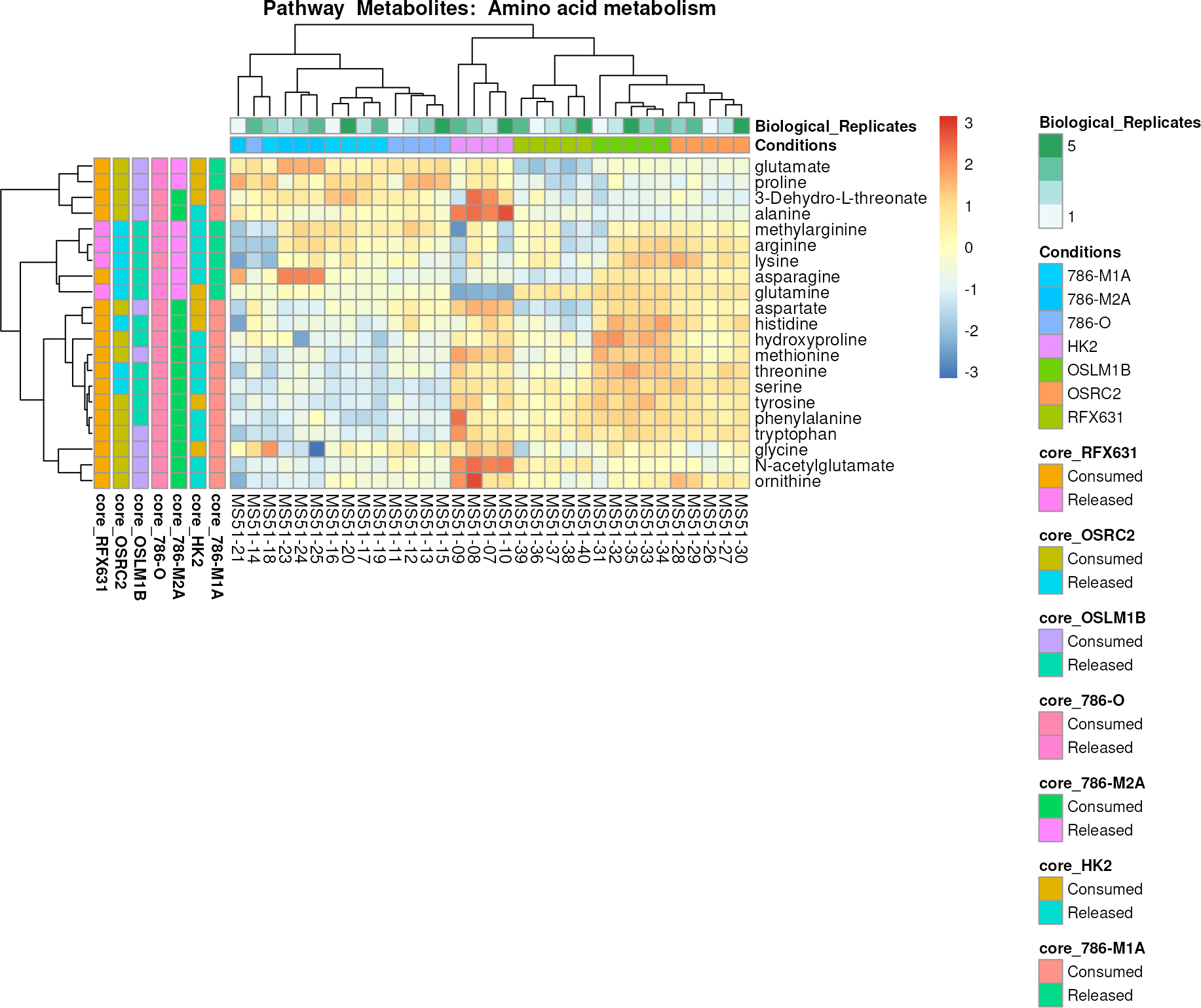
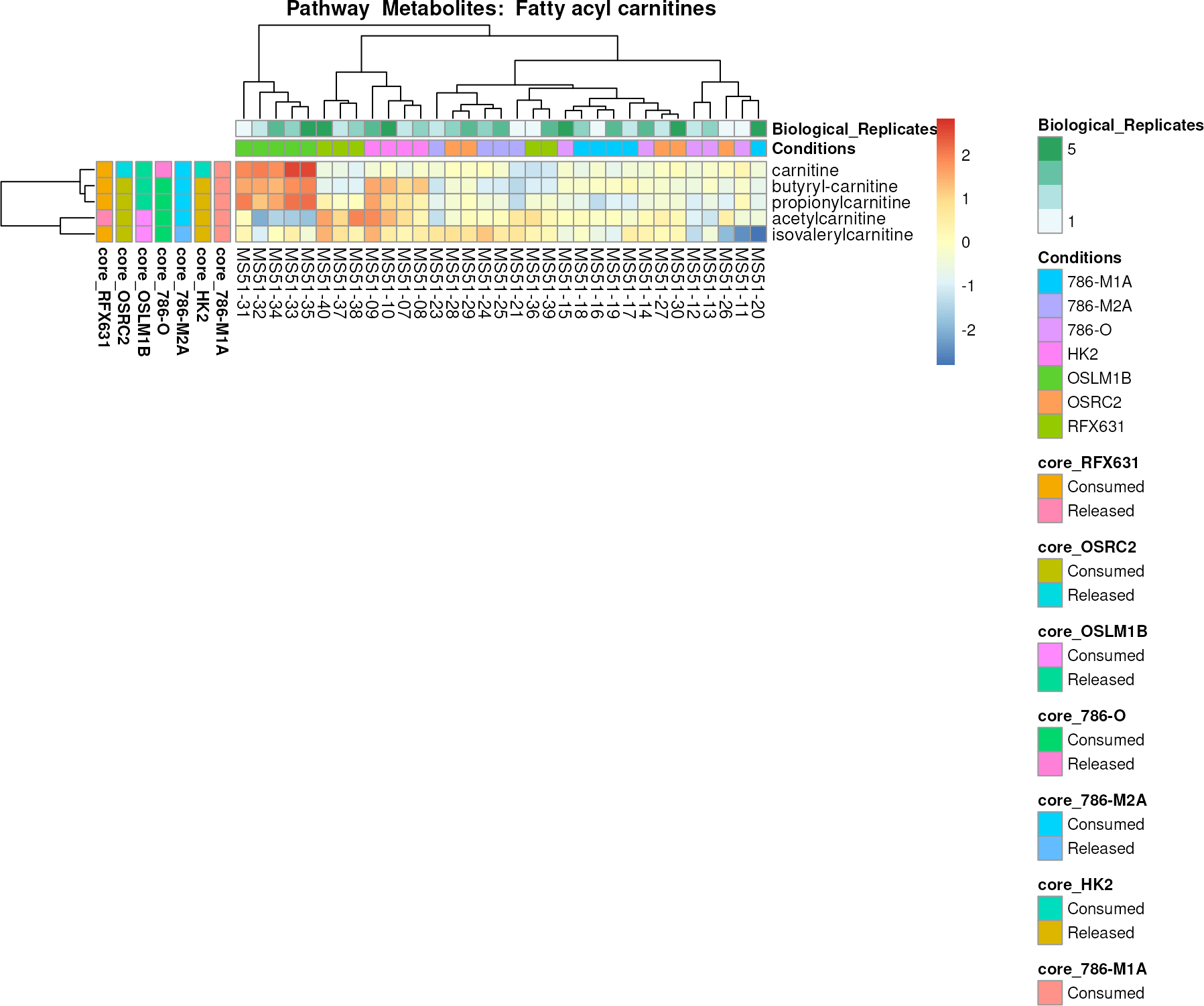
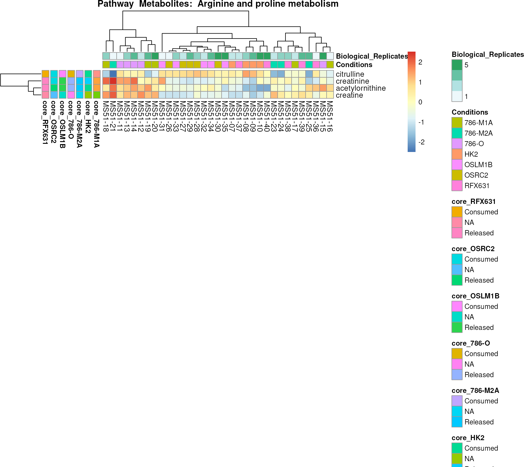
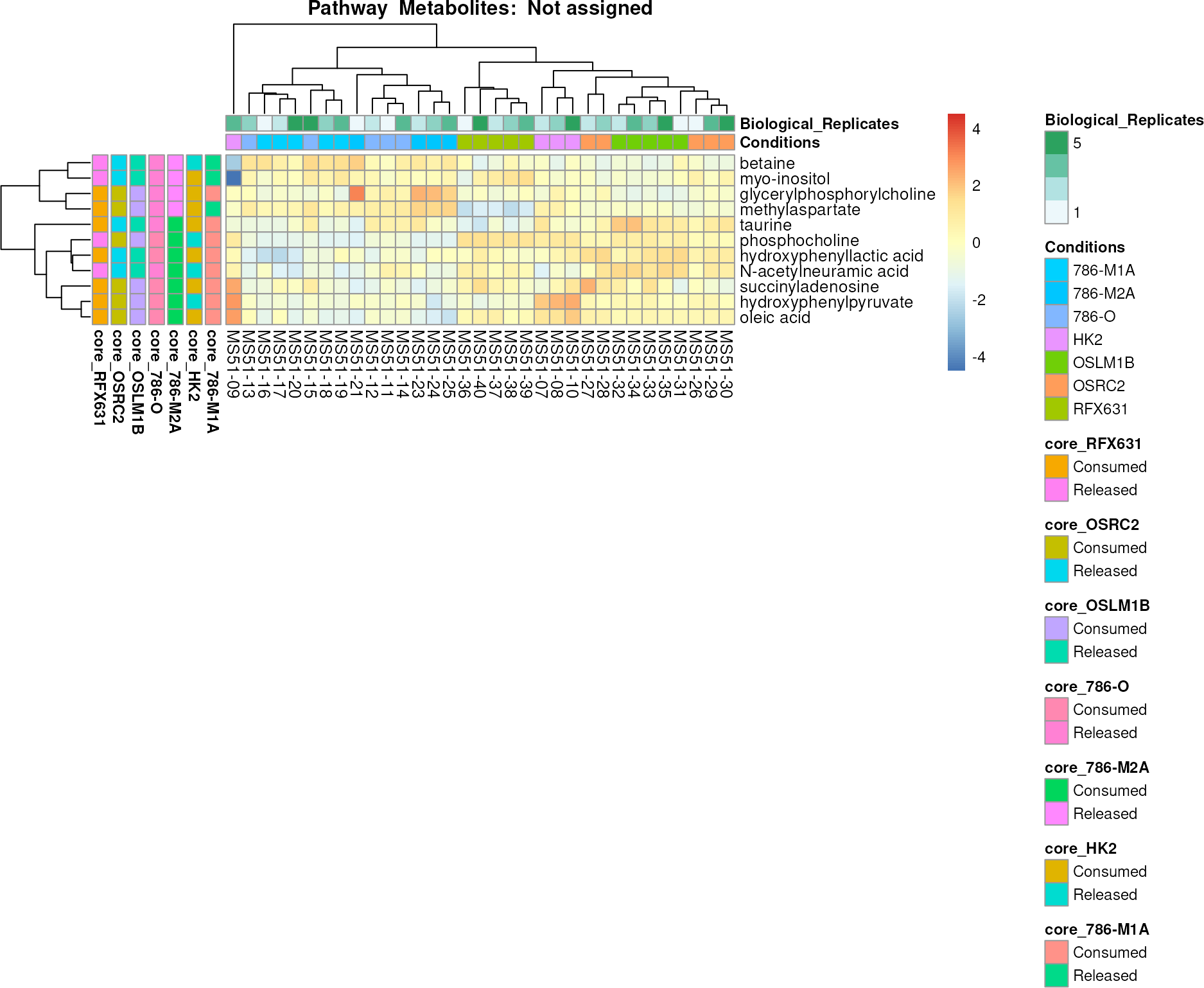
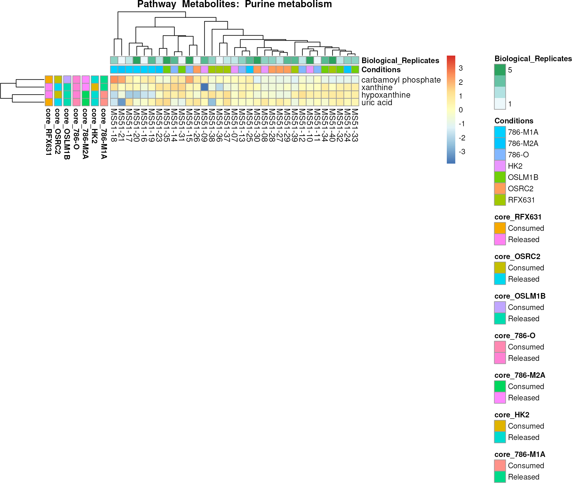
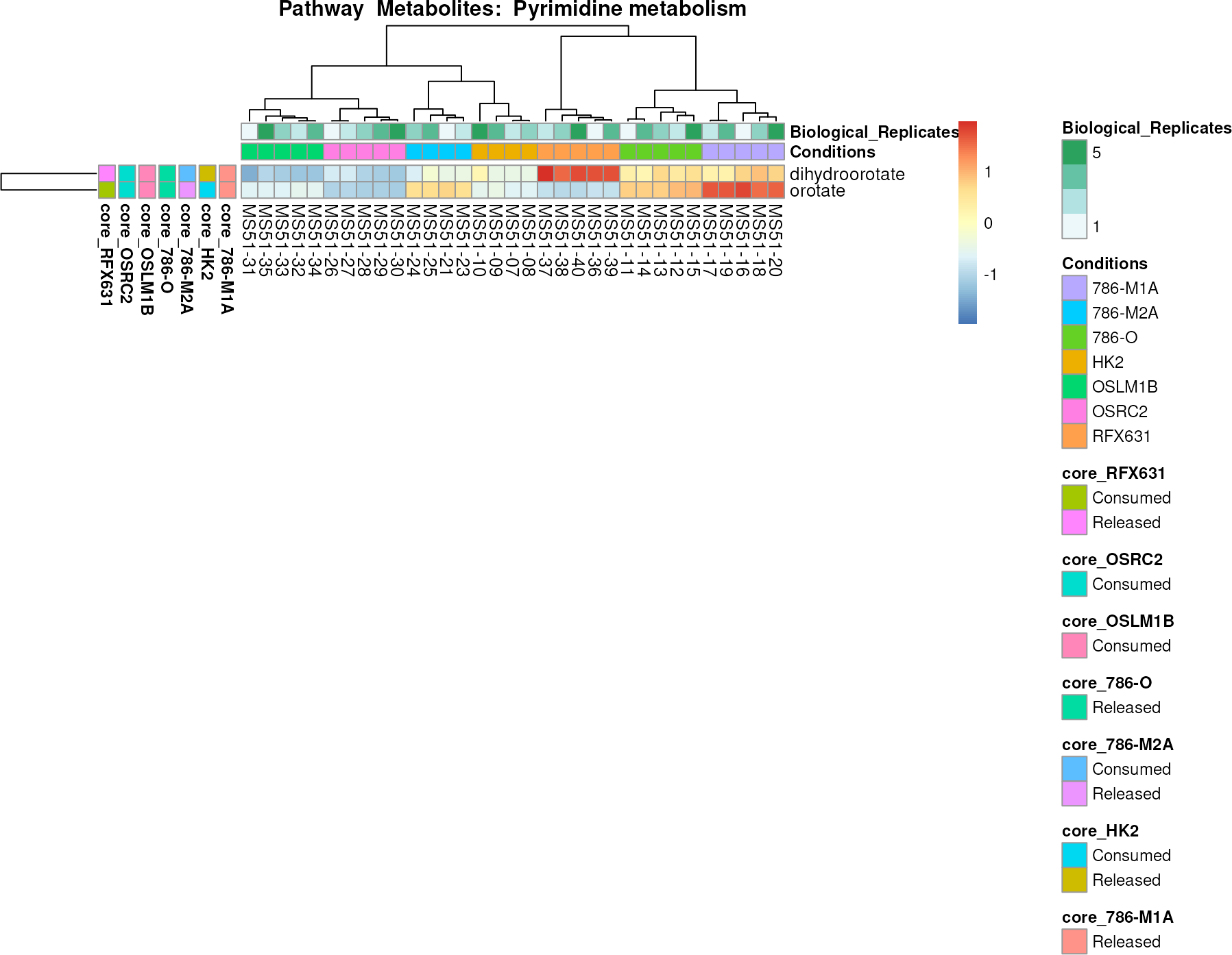
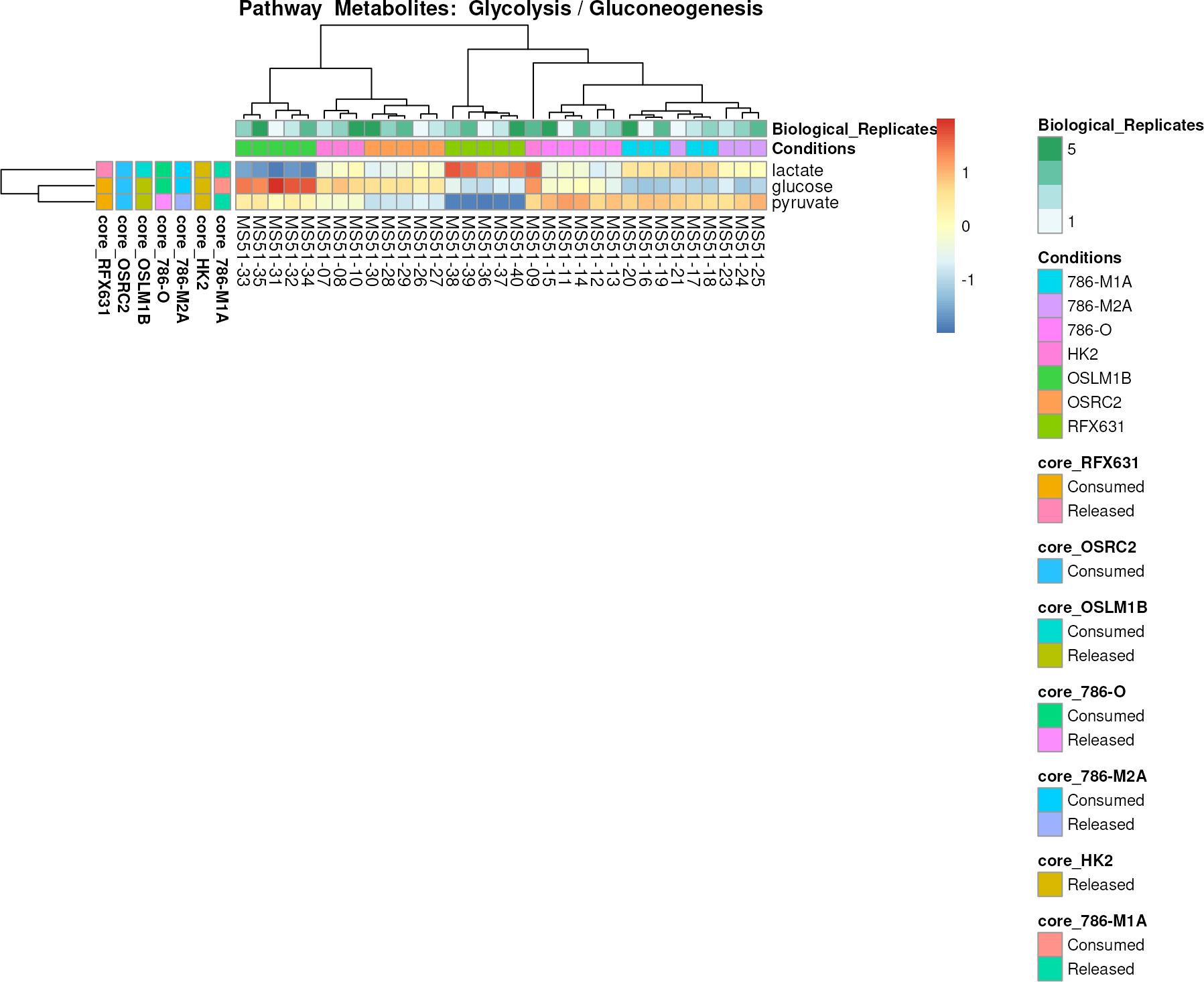
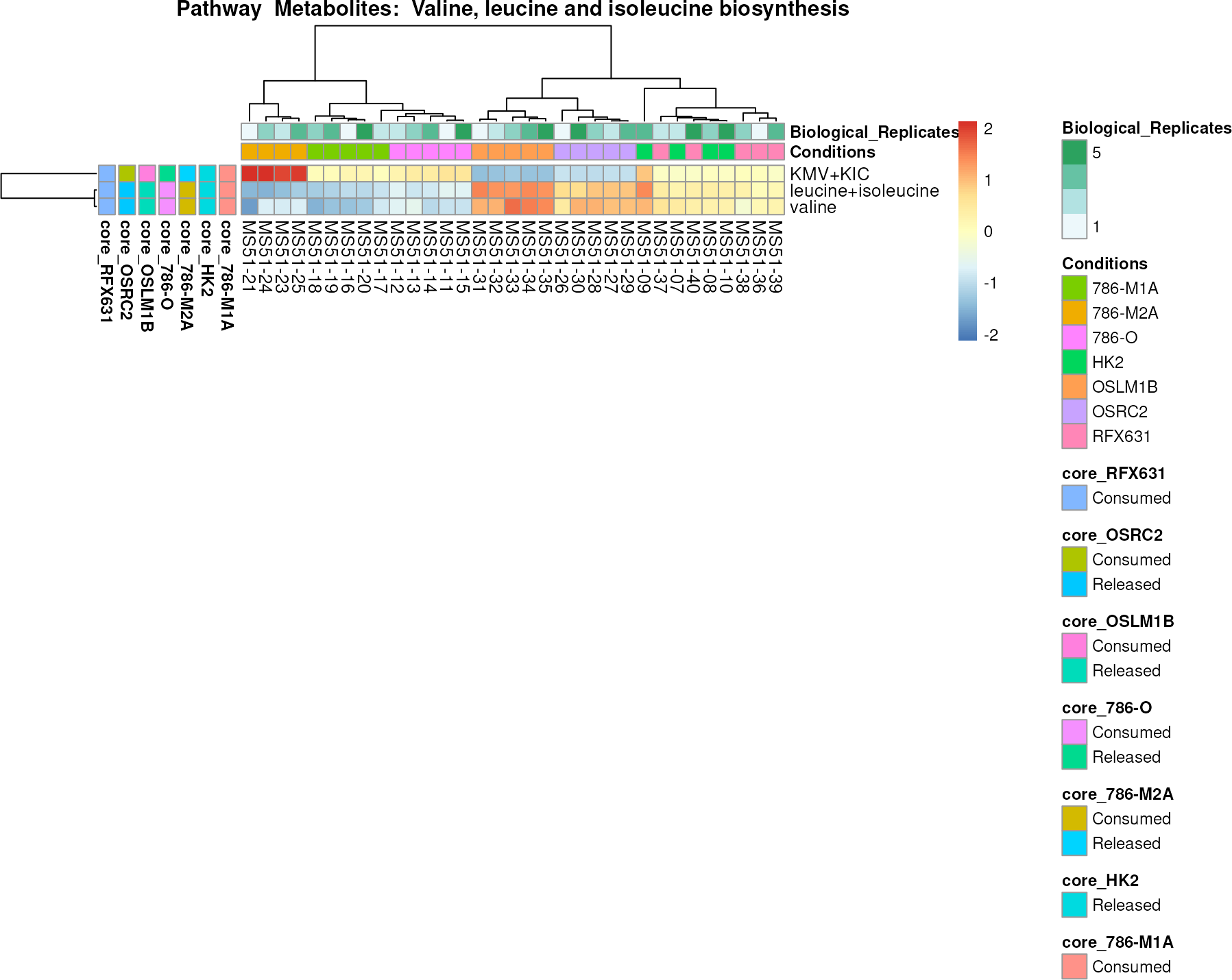
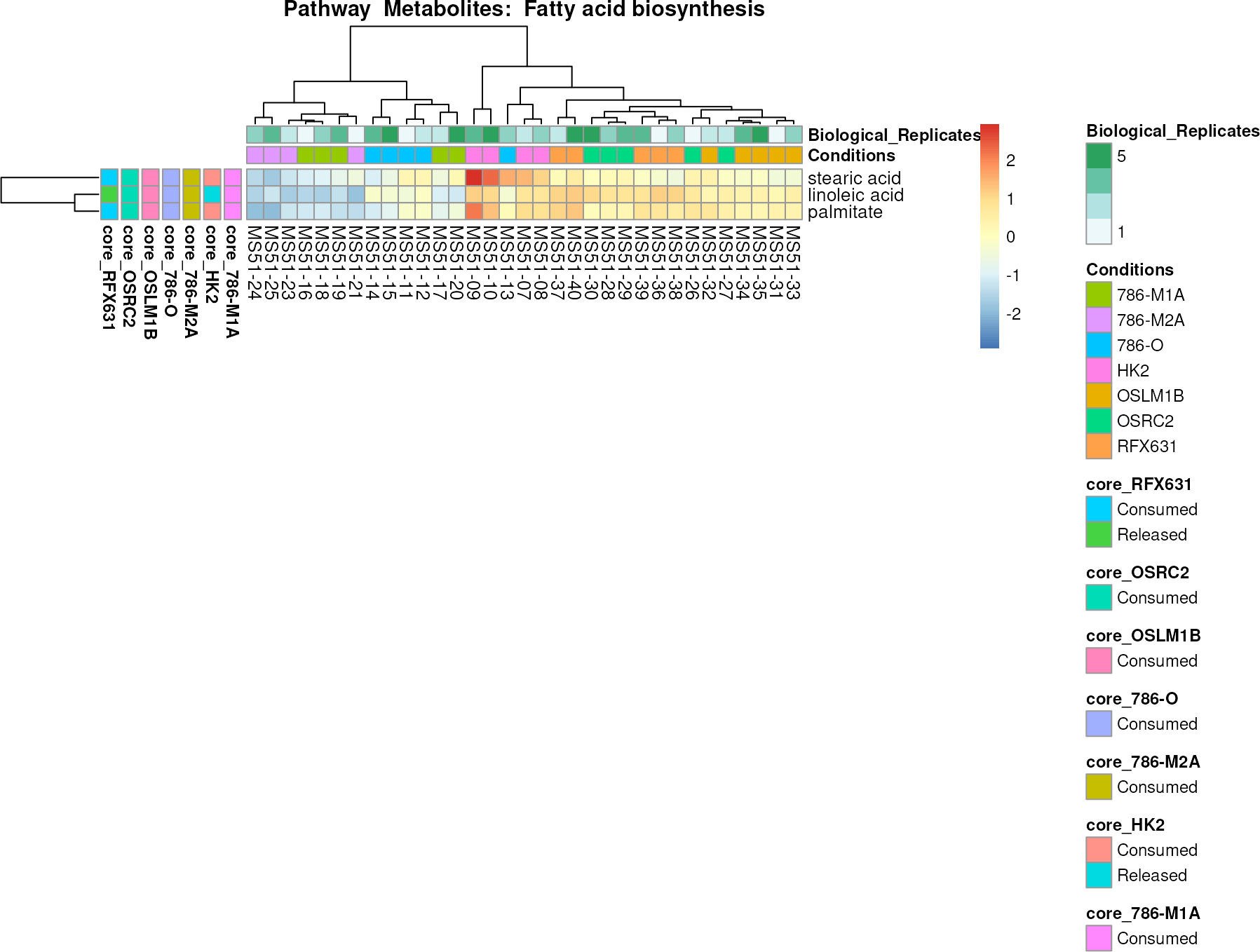
Lastly, by generating individual plots for e.g. each pathway or the metabolite clusters by adding individual (individual_Sample or individual_Metab) to metadata_info. At the same time we can still maintain the metadata information for both, the samples and the metabolites. Together this can help us to draw biological conclusions about the different pathways: Indeed, we can observe for the D-Amino acid metabolism many metabolites fall into the MCA-Cluster core_DOWN, meaning in comparison to HK2 cells we have a negative Log2FC for 786-O and 786-M1A.

viz_heatmap(data = Input_Heatmap,
metadata_sample = MetaData_Sample,
metadata_info = c(individual_Metab = "Pathway",
                                        color_Sample = list("Conditions","Biological_Replicates"),
                                        color_Metab = list("core_786-M1A", "core_HK2", "core_786-M2A", "core_786-O", "core_OSLM1B", "core_OSRC2", "core_RFX631")),
                                        metadata_feature =  MetaData_Metab,
                                        plot_name = "Pathway")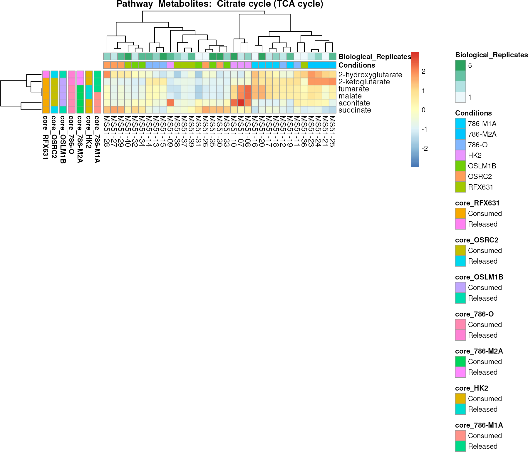

You can also choose to make individual plots for any Sample Metadata using individual_Sample (e.g. in patients you may want to plot male and female separately). Moreover, you can also use both at the same time.

Superplots

Sometimes one might be interested to create individual plots for each metabolite to understand the differences between specific conditions. For this common plot types are bargraphs, boxplots or violin plots. As input, we need a DF that contains the samples as rownames and the features (=metabolites) as column names:

Input_Superplot <-  Media_Preprocessed[,-c(1:4)]#remove columns that include Metadata such as cell type,...

Input for viz_superplot(), with samples as rownames and metabolites as column names.

	valine-d8	hipppuric acid-d5	2-hydroxyglutarate	2-ketoglutarate	3-Dehydro-L-threonate	acetylcarnitine	acetylcholine
MS51-07	5049281744	30218506574	-868601575	1530912430	28673393701	-67547592848	-496576017
MS51-08	-1441406385	-11561761745	1108346025	3684365990	39313101752	-234677799645	-124297109
MS51-09	2563904070	-10237061776	-189633550	-9097094735	-67782920598	218513442831	526295913
MS51-10	-6171779428	-8419683053	-50110899	3881816314	-203574855	83711949661	94577213
MS51-11	27378617230	123649127347	4311754839	23286535748	-16721754062	-434945308541	-183109349
MS51-12	31998154622	99965859879	808357705	19381509727	-16349278172	-583665678018	-998475065
MS51-13	26220971337	99972874145	-235593734	19536285942	-28131696536	-645802166950	-822951440
MS51-14	27882417489	115689376712	1115432087	17101698081	-26309877624	-275257639669	-1272434260
MS51-15	24806237271	132343157722	-1179339178	17846663766	-40351828895	-321374884275	-1318142384
MS51-16	11094140749	57354194293	5445671697	28056643231	9905712215	-356638276041	-929117918
MS51-17	34144526544	116670253290	3041583921	22341957663	-1871784883	-379917701289	-1217951807
MS51-18	30843226841	131915991104	2364979960	19876068811	-12106631836	-297445077871	-907725948
MS51-19	26032777849	93842230196	600387750	22338213828	-15996801077	-325213646459	-1216114751
MS51-20	15413411654	47939629182	4007911817	20555474456	13695406411	-438100232873	-1430510133
MS51-21	53001553101	127450060294	4809729749	39166236259	-38896232803	-125539074625	-943874817
MS51-23	47001796040	161667174110	6707051392	38517108736	-6979130432	-673387467221	-664880164
MS51-24	8217942926	37130736106	5857701472	39276732227	-10740427138	-333936377093	-1206364609
MS51-25	7242347148	57539536462	4568079831	40583987397	-18377163802	-282195052525	-1314339238
MS51-26	1631567949	36681096085	1121378276	-2694080144	-60644185117	-198965081888	-843128099
MS51-27	1209476862	-8930444074	3405336890	-2060735139	-51783244894	-209186167980	-365874316
MS51-28	-4518925715	-2435870916	7007395646	-2525310574	-30952324005	-408114545906	-609942826
MS51-29	1484077336	-2058725307	3515115140	-5164411612	-42307838881	-287356849930	-912778912
MS51-30	4368619286	15502685767	-1093856576	-4703700433	-60704125766	-260908005179	-383882500
MS51-31	7907484382	12534261776	-2452294215	-8563910085	-75125518110	-289811675340	-918369787
MS51-32	10026207227	8766901671	1953315759	-7520737233	-55168263224	-890597864901	-314644061
MS51-33	1320088121	-19794580878	-541809575	-6750277825	-52231898984	-770337735939	-182991027
MS51-34	4019534162	-21662185450	1428924068	-7578531520	-47605477000	-741976996697	-550044215
MS51-35	-11674356179	-75718957578	972005613	-6094793780	-57165852971	-822161480737	-503488121
MS51-36	9892941550	46138316334	4954019648	5560697649	-23867649475	-71475573825	-1119704368
MS51-37	14414593887	78736973172	-257560661	-2341634721	-51914744178	-35405004462	-687055540
MS51-38	7716702900	3492507671	-2307137058	-4331637640	-67900220172	230840109765	-408157136
MS51-39	-583337199	-9483365742	706088109	-2757559248	-56366820622	-263196399957	-227087862
MS51-40	11097184979	24818171463	3186690665	-4462779576	-50563367720	145901488878	-319389629

We also need the Metadata as we will need to know which conditions to plot for together. If you have further information such as replicates or patient ID, we can use this for the colour of the plotted samples per condition as in the superplots style as described in by Lord et al (Lord et al. 2020).

metabolite_list <- MCA_res %>%
filter(stringr::str_detect(RG2_Significant, "Opposite"))%>%
pull(Metabolite)


viz_superplot(data =Input_Superplot%>%  select(any_of(metabolite_list)),#We just plot selected metabolites
metadata_sample =MetaData_Sample,
metadata_info = c(Conditions="Conditions", Superplot = "Biological_Replicates"),
plot_type = "Bar", #Bar, Box, Violin
plot_conditions = c("HK2", "786-O", "786-M1A", "786-M2A", "OSRC2", "OSLM1B", "RFX631"),#sets the order in which the samples should be plotted
stat_comparison = list(c(1,2),c(1,4)))#Stat comparisons to be included on the plot
#> Ignoring unknown labels:
#> • fill : "Biological_Replicates"
#> Ignoring unknown labels:
#> • fill : "Biological_Replicates"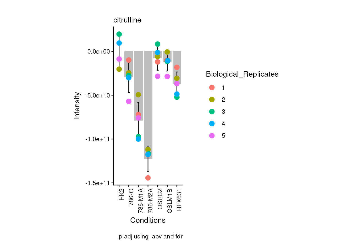

#> Ignoring unknown labels:
#> • fill : "Biological_Replicates"
#> Ignoring unknown labels:
#> • fill : "Biological_Replicates"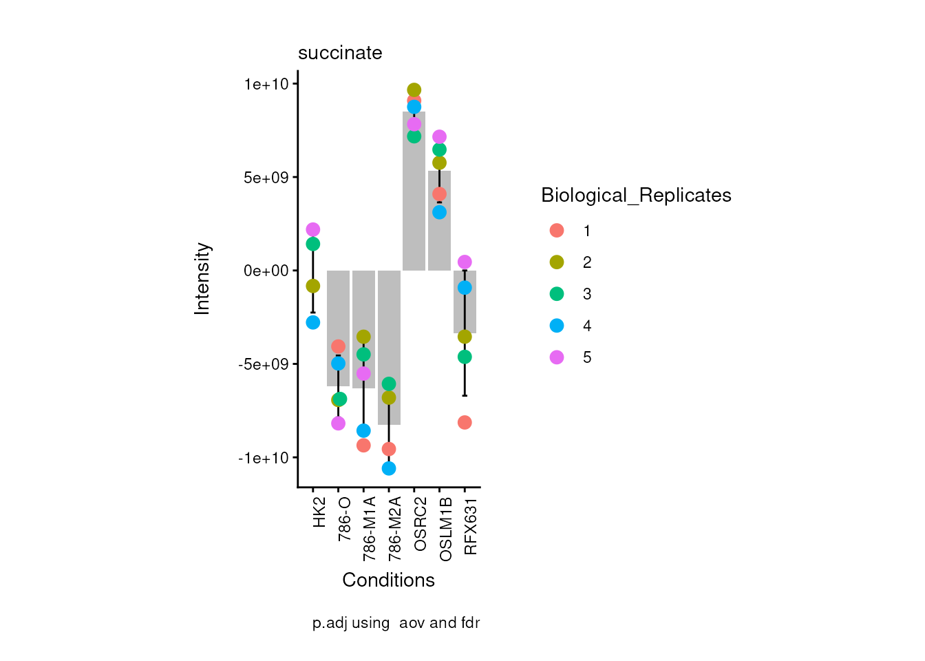

Now, if we for instance prefer boxplots over bargraphs we can simply change the parameter plot_type:

viz_superplot(data =Input_Superplot[,c(1:6)],#We just plot six metabolites
metadata_sample =MetaData_Sample,
metadata_info = c(Conditions="Conditions", Superplot = "Biological_Replicates"),
plot_type = "Box", #Bar, Box, Violin
plot_conditions = c("HK2", "786-O", "786-M1A", "786-M2A", "OSRC2", "OSLM1B", "RFX631"),#sets the order in which the samples should be plotted
stat_comparison = list(c(1,2),c(1,4)))#Stat comparisons to be included on the plot
#> Ignoring unknown labels:
#> • fill : "Biological_Replicates"
#> Ignoring unknown labels:
#> • fill : "Biological_Replicates"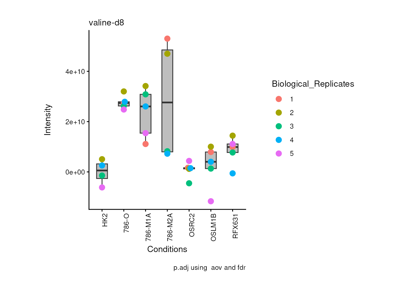

#> Ignoring unknown labels:
#> • fill : "Biological_Replicates"
#> Ignoring unknown labels:
#> • fill : "Biological_Replicates"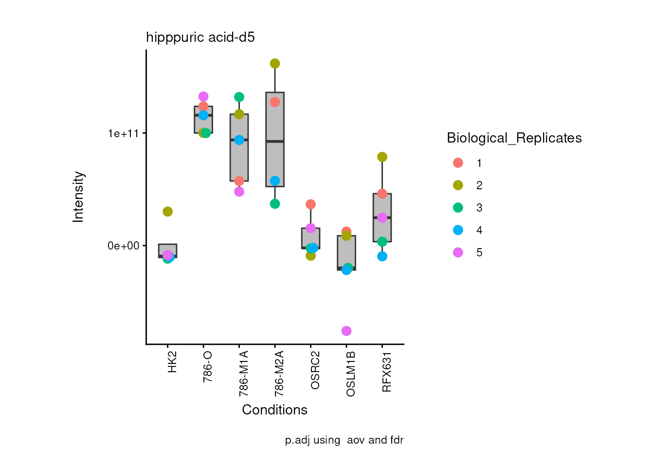

#> Ignoring unknown labels:
#> • fill : "Biological_Replicates"
#> Ignoring unknown labels:
#> • fill : "Biological_Replicates"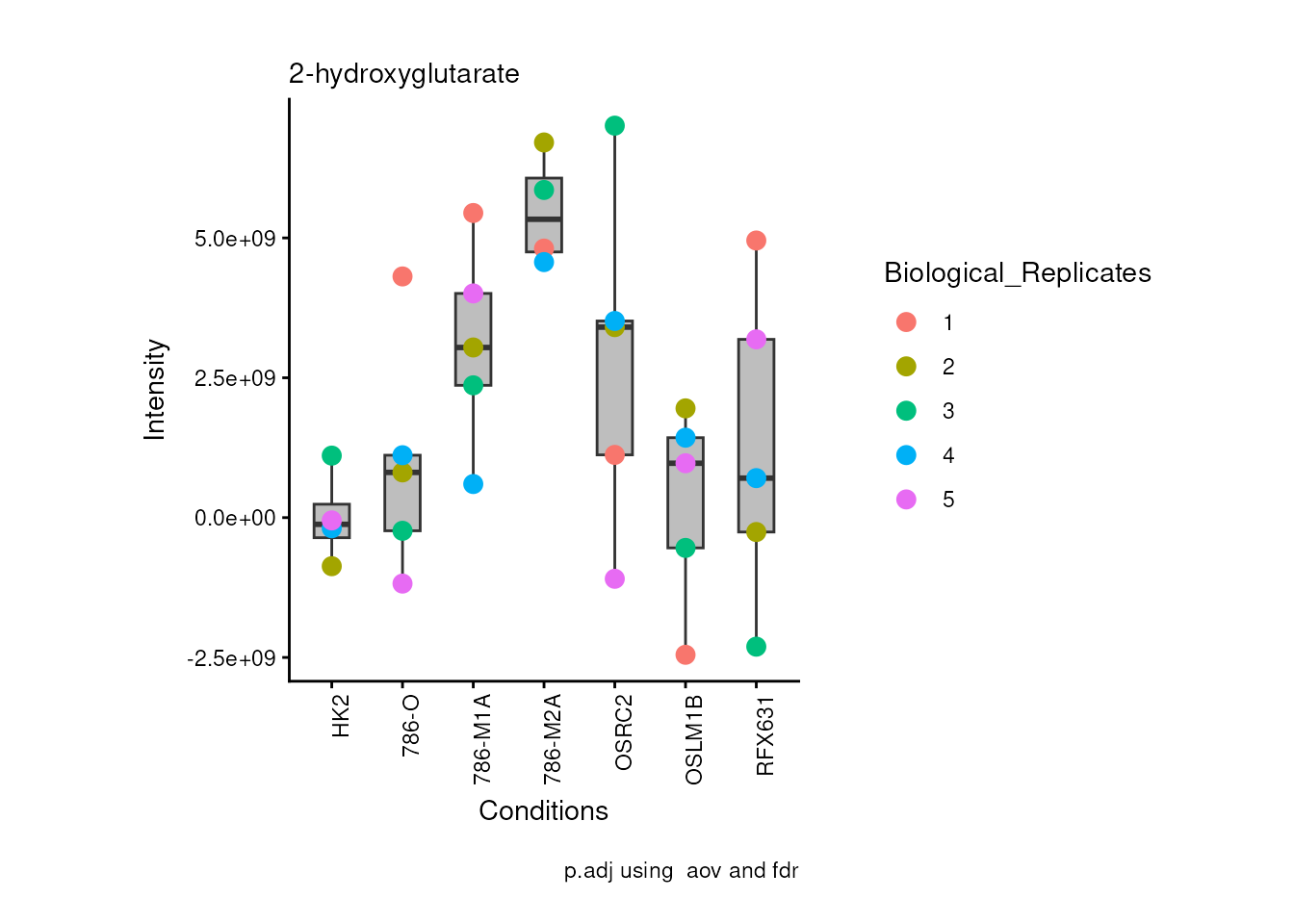

#> Ignoring unknown labels:
#> • fill : "Biological_Replicates"
#> Ignoring unknown labels:
#> • fill : "Biological_Replicates"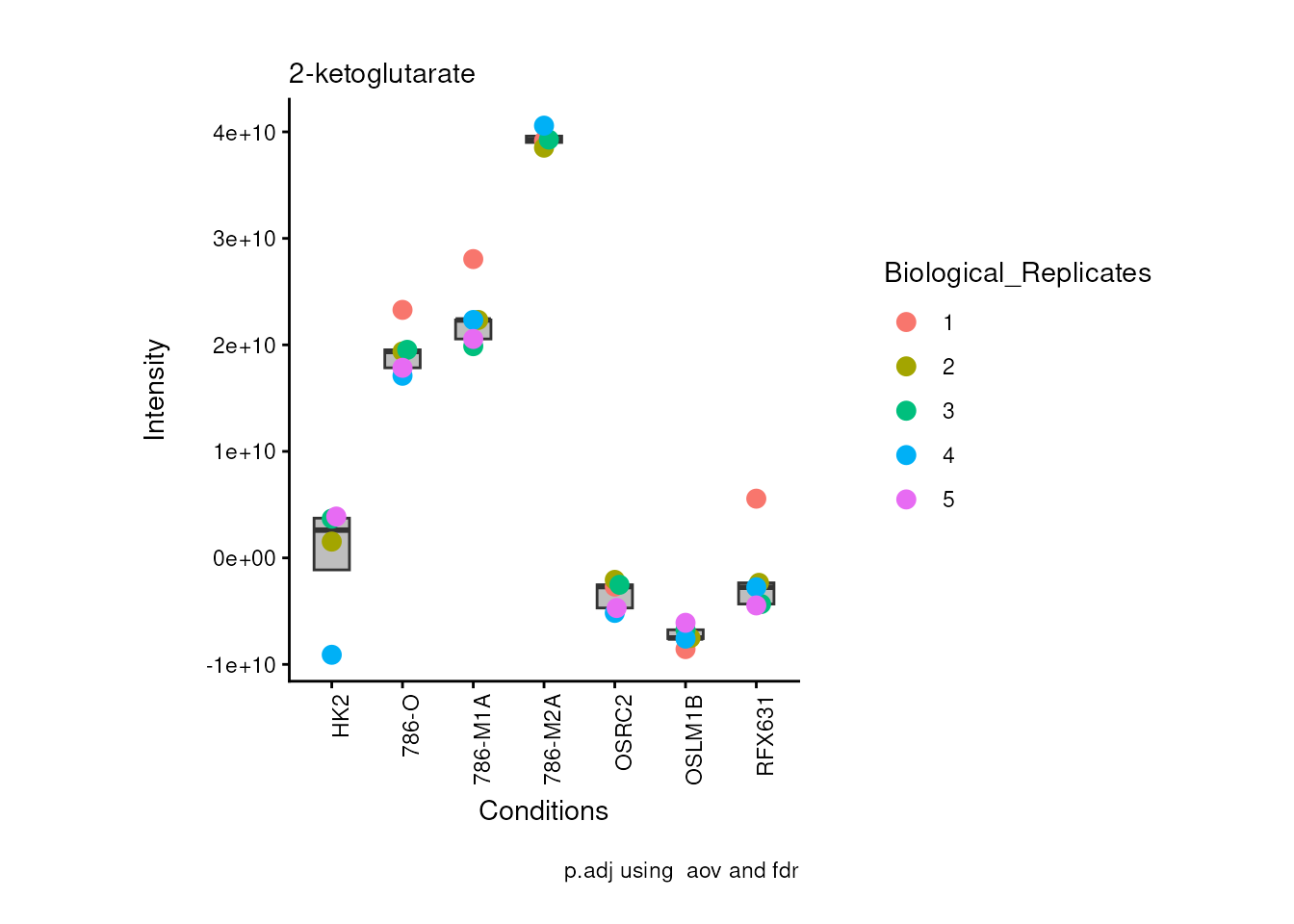

#> Ignoring unknown labels:
#> • fill : "Biological_Replicates"
#> Ignoring unknown labels:
#> • fill : "Biological_Replicates"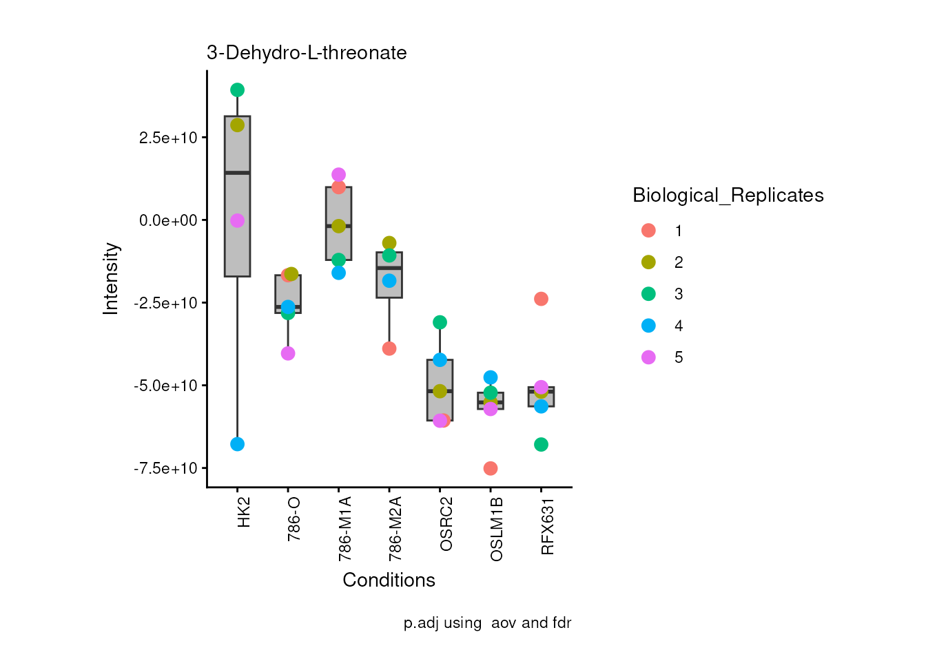

#> Ignoring unknown labels:
#> • fill : "Biological_Replicates"
#> Ignoring unknown labels:
#> • fill : "Biological_Replicates"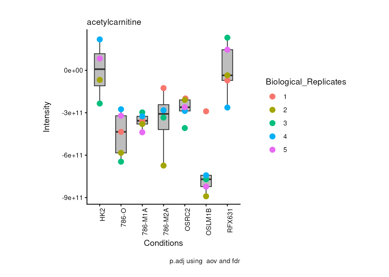

We can also change it to violin plots:

viz_superplot(data =Input_Superplot[,c(1:6)],#We just plot six metabolites
metadata_sample =MetaData_Sample,
metadata_info = c(Conditions="Conditions", Superplot = "Biological_Replicates"),
plot_type = "Violin", #Bar, Box, Violin
plot_conditions = c("HK2", "786-O", "786-M1A", "786-M2A", "OSRC2", "OSLM1B", "RFX631"),#sets the order in which the samples should be plotted
stat_comparison = list(c(1,2),c(1,4)))#Stat comparisons to be included on the plot
#> Ignoring unknown labels:
#> • fill : "Biological_Replicates"
#> Ignoring unknown labels:
#> • fill : "Biological_Replicates"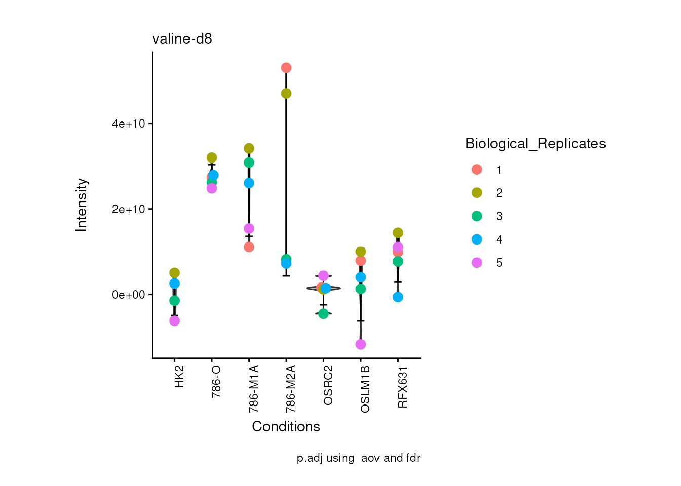

#> Ignoring unknown labels:
#> • fill : "Biological_Replicates"
#> Ignoring unknown labels:
#> • fill : "Biological_Replicates"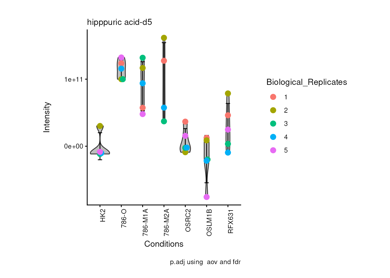

#> Ignoring unknown labels:
#> • fill : "Biological_Replicates"
#> Ignoring unknown labels:
#> • fill : "Biological_Replicates"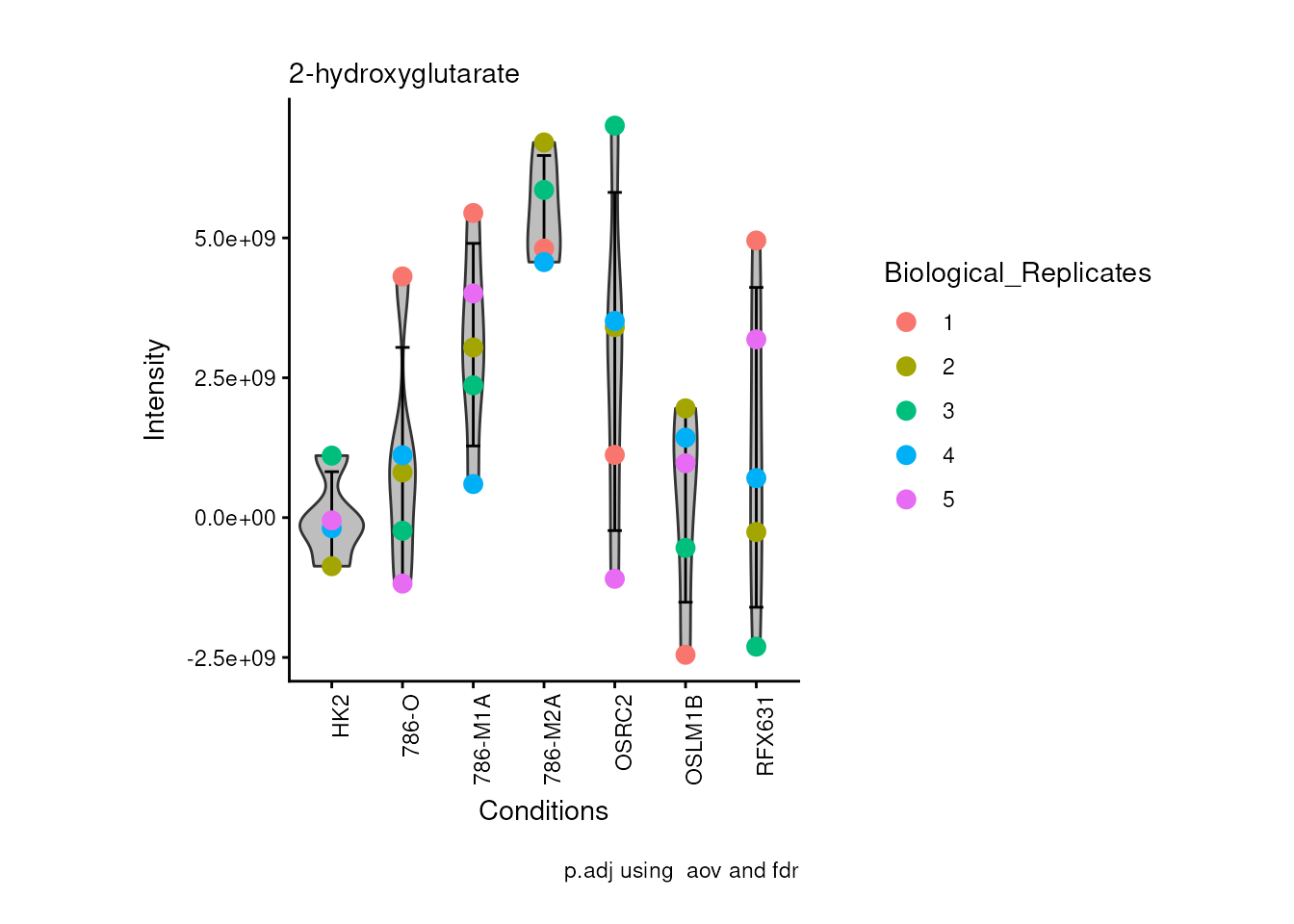

#> Ignoring unknown labels:
#> • fill : "Biological_Replicates"
#> Ignoring unknown labels:
#> • fill : "Biological_Replicates"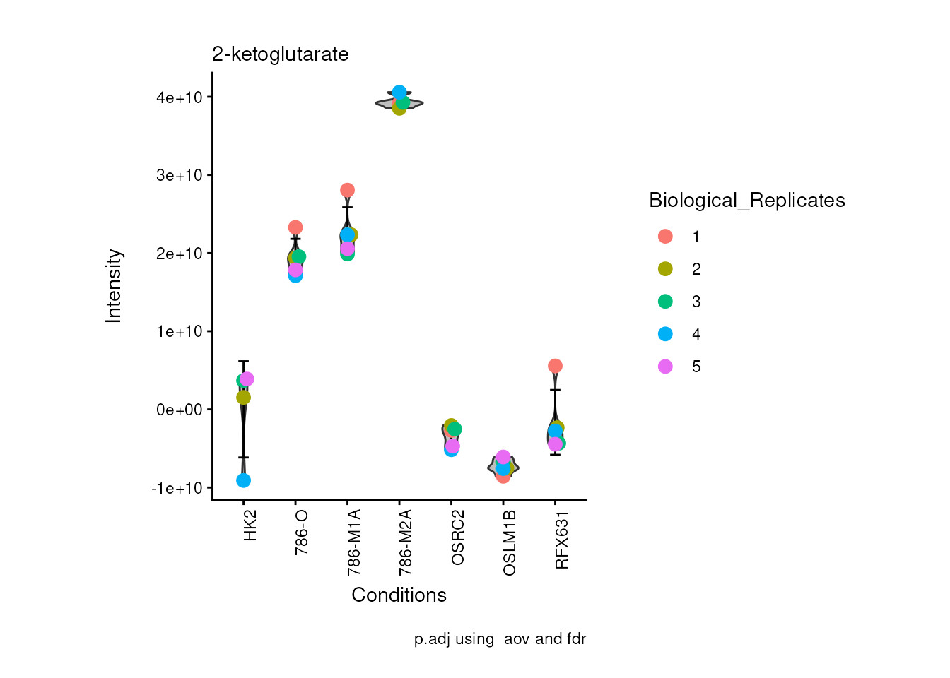

#> Ignoring unknown labels:
#> • fill : "Biological_Replicates"
#> Ignoring unknown labels:
#> • fill : "Biological_Replicates"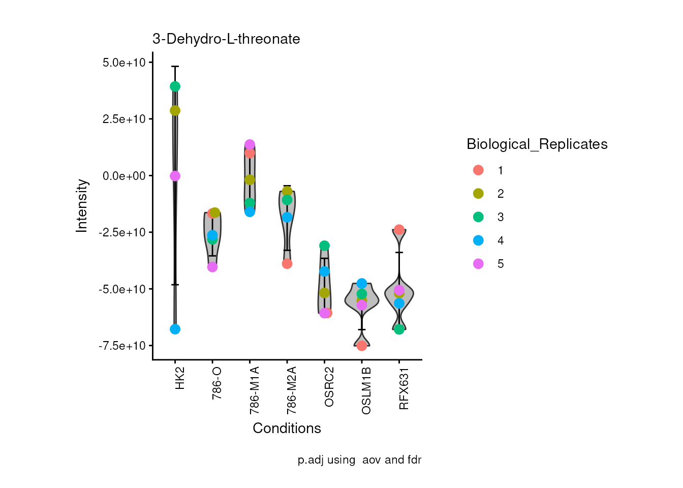

#> Ignoring unknown labels:
#> • fill : "Biological_Replicates"
#> Ignoring unknown labels:
#> • fill : "Biological_Replicates"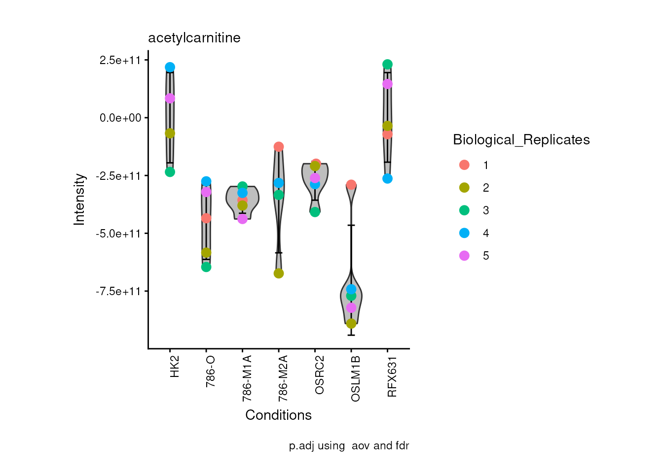

Volcano plot

In general, viz_volcano() has three different plot types, which are set with the parameter plot_types:
1. "Standard" is the standard version of the plot, with one dataset being plotted.
2. "Compare" here two datasets (data and data2) will be plotted together.
3. "PEA" stands for Pathway Enrichment Analysis, and is used if the results of an GSE analysis should be plotted as here the figure legends will be adapted. You can find an example for this in the vignette Standard Metabolomics

Here we will look at all the different options we have to display our results from the different analysis, which will help us to interpret our results as this can be sometimes difficult to do from the many data tables.
Just a quick reminder, how the input data look like:
1. Results of Differential Metabolite Analysis (dma): Log2(Distance) and stats:

Input data for viz_volcano() are for example differential analysis results from dma().

Metabolite	Log2(Distance)	p.adj	t.val	Mean_786-M1A	core_786-M1A
2-hydroxyglutarate	-31.52594	0.3447870	-3092107029	3092107028.86536	Released
2-ketoglutarate	-34.39775	0.0000000	-22633671598	22633671597.7763	Released
3-Dehydro-L-threonate	30.24765	0.9999999	1274819834	-1274819834.18323	Consumed
acetylcarnitine	38.38705	0.0653736	359462986907	-359462986906.515	Consumed
acetylcholine	30.08675	0.0004996	1140284111	-1140284111.31361	Consumed
acetylornithine	-32.65274	0.0012793	-6752323351	6752323351.13854	Released
aconitate	32.58145	0.0000000	6426780519	-6426780518.51619	Consumed

Standard

Here we will first look into the results from the differential analysis (see section dma above) for the comparison of HK2_vs_786M1A:

# Run with default parameters --> we only need to provide the data
viz_volcano(data=DMA_HK2_vs_786M1A%>%column_to_rownames("Metabolite"),
x= "Log2(Distance)")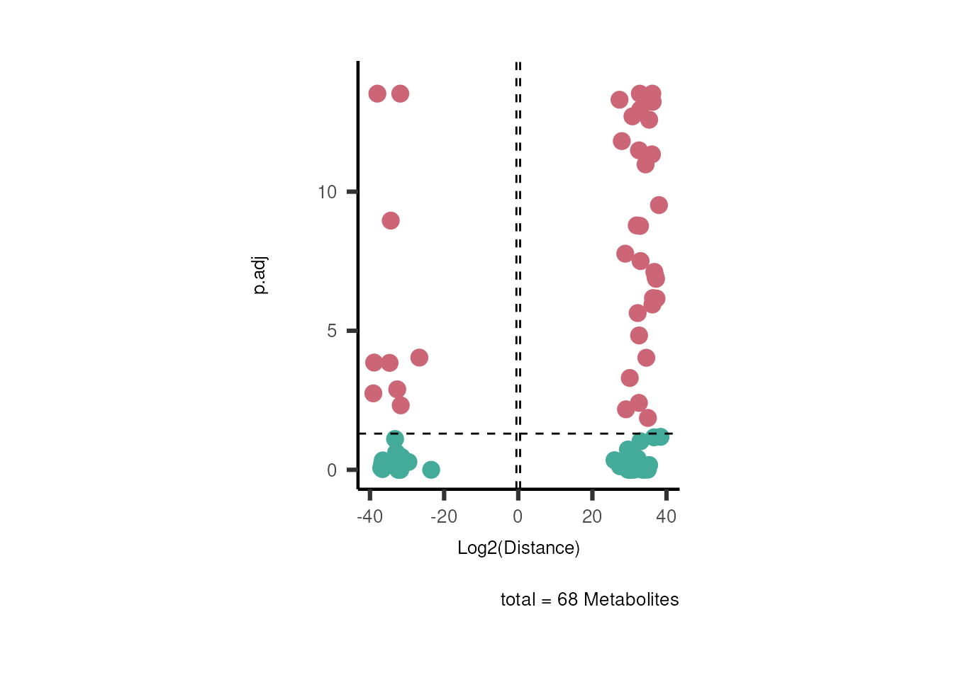

Standard figure displaying dma results.

If you seek to plot the metabolite names you can change the parameter select_label from its default (select_label="") to NULL and the metabolite names will be plotted randomly.

# Run with default parameters --> we only need to provide the data
viz_volcano(data=DMA_HK2_vs_786M1A%>%column_to_rownames("Metabolite"),
x= "Log2(Distance)",
select_label = NULL)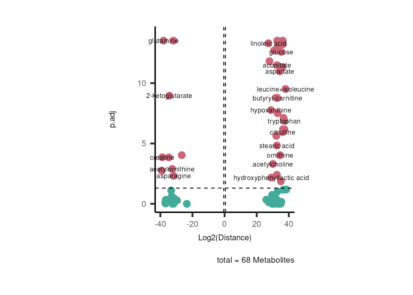

Standard figure displaying dma results.

With the parameter select_label you can also pass a vector with Metabolite names that should be labeled:

# Run with default parameters --> we only need to provide the data
viz_volcano(data=DMA_HK2_vs_786M1A%>%column_to_rownames("Metabolite"),
x= "Log2(Distance)",
select_label = c("histidine", "phenylalanine", "lactate"))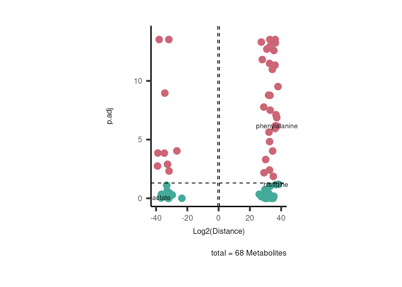

Standard figure displaying dma results.

As explained above, when analyzing core data it is important to take into account if a metabolite is consumed or released. we can use this information to colour code and or shape the metabolites on the plot.
For this we need to add this information into the Metadata_Metabolite file:

# colour for consumption and release: For this we need to add this information into the Metadata_Metabolite file
MetaData_Metab <- merge(MappingInfo%>%rownames_to_column("Metabolite"), DMA_HK2_vs_786M1A[,c(1,6,8:10)], by="Metabolite", all.y=TRUE)%>%
column_to_rownames("Metabolite")

Metadata table including additional information about the Metabolites.

	HMDB	KEGG.ID	KEGGCompound	Pathway	core_786-M1A	core_HK2	core_specific	core
3-Dehydro-L-threonate	NA	NA	NA	Amino acid metabolism	Consumed	Consumed	Consumed	Consumed
acetylcarnitine	HMDB0000201	C02571	O-Acetylcarnitine	Fatty acyl carnitines	Consumed	Released	Consumed in 786-M1A and Released HK2	Released / Consumed
acetylornithine	HMDB0003357	C00437	N-Acetylornithine	Arginine and proline metabolism	Released	Consumed	Released in 786-M1A and Consumed HK2	Released / Consumed
glutamate	HMDB0000148	C00025	L-Glutamate	Amino acid metabolism	Released	Consumed	Released in 786-M1A and Consumed HK2	Released / Consumed
glutamine	HMDB0000641	C00064	L-Glutamine	Amino acid metabolism	Released	Consumed	Released in 786-M1A and Consumed HK2	Released / Consumed
glycerylphosphorylcholine	HMDB0252858	NA	NA	Not assigned	Consumed	Consumed	Consumed	Consumed

Now we can make the different plots:

# Now we need to add our metadata_feature and metadata_info:
viz_volcano(plot_types="Standard",
metadata_info= c(color="core_specific"),
metadata_feature= MetaData_Metab,
data=DMA_HK2_vs_786M1A%>%column_to_rownames("Metabolite"),
x= "Log2(Distance)",
plot_name= "786M1A versus HK2",
subtitle= "Results of dma. Colour coded for consumption/release" )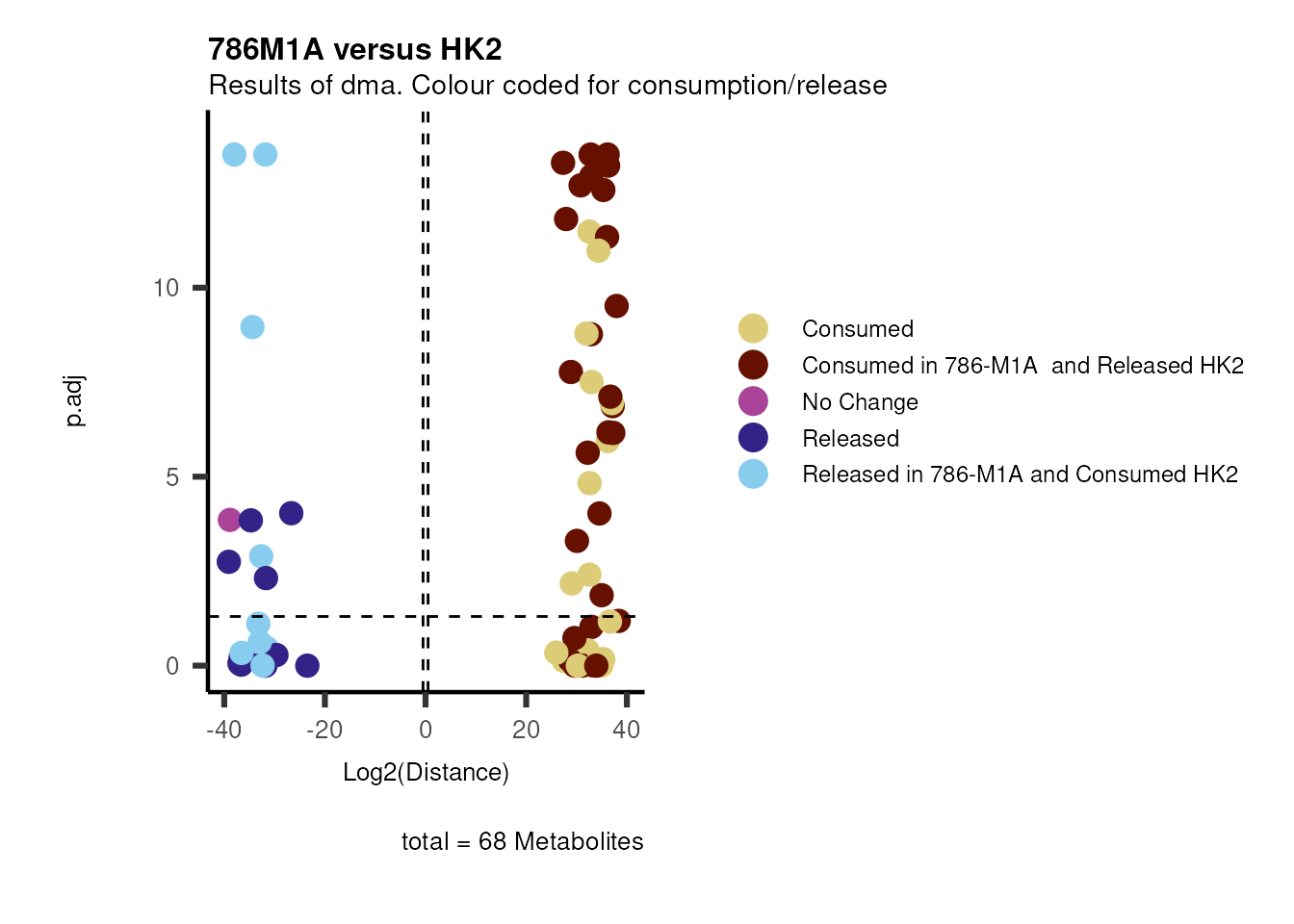

Standard figure displaying dma results.

# If we want to use the shape instead of the colour for the cluster info, we can just change our metadata_info
viz_volcano(plot_types="Standard",
metadata_info= c(shape="core_specific"),
metadata_feature= MetaData_Metab,
data=DMA_HK2_vs_786M1A%>%column_to_rownames("Metabolite"),
x= "Log2(Distance)",
plot_name= "786M1A versus HK2",
subtitle= "Results of dma. Shape for consumption/release, color for significance." )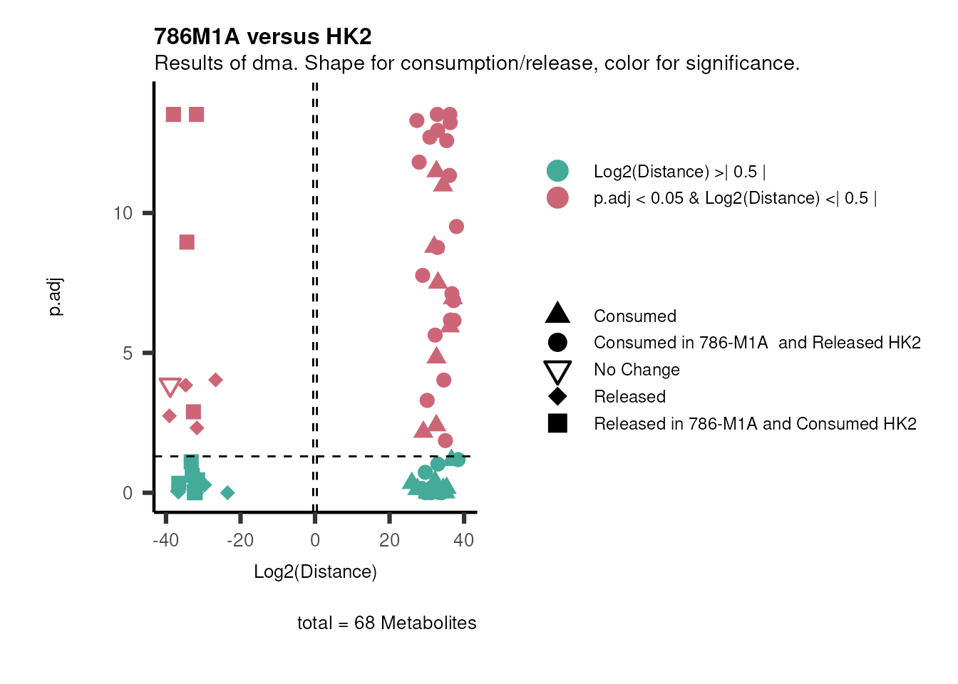

Standard figure displaying dma results.

# Of course, we can also adapt both, color and shape for the same parameter:
viz_volcano(plot_types="Standard",
metadata_info= c(shape="core_specific", color="core_specific"),
metadata_feature= MetaData_Metab,
data=DMA_HK2_vs_786M1A%>%column_to_rownames("Metabolite"),
x= "Log2(Distance)",
plot_name= "786M1A versus HK2",
subtitle= "Results of dma. Shape and color for consumption/release." )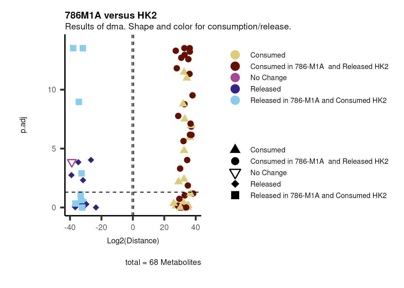

Standard figure displaying dma results.

Of course, here we may also want an individual plot for each of the consumption/release metabolites.

# individual plot for each metabolite behaviour:
viz_volcano(plot_types="Standard",
metadata_info= c(individual="core", shape="core_specific"),
metadata_feature= MetaData_Metab,
data=DMA_HK2_vs_786M1A%>%column_to_rownames("Metabolite"),
x= "Log2(Distance)",
plot_name= "786M1A versus HK2",
subtitle= "Results of dma." )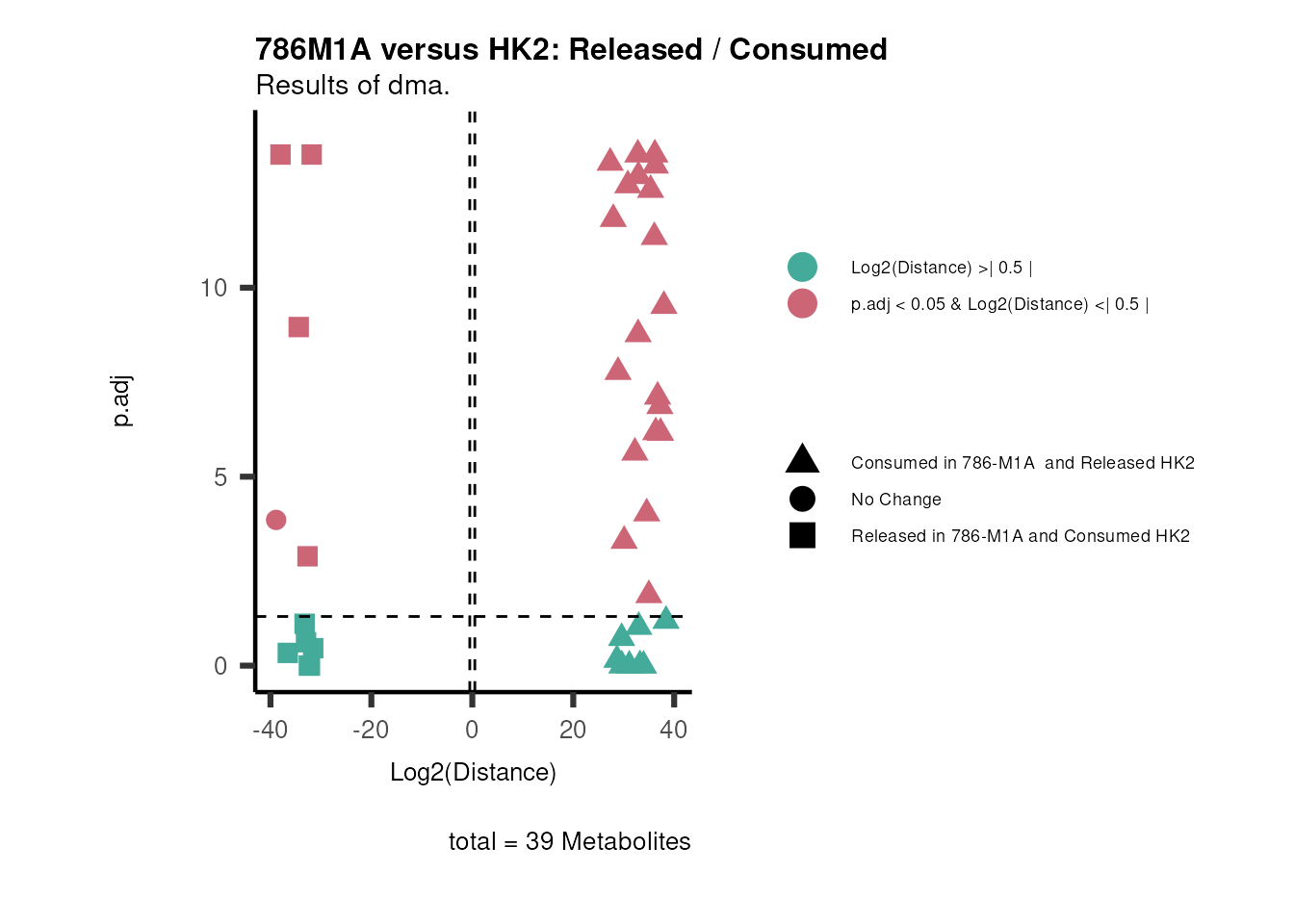

Standard figure displaying dma results.

#> Warning: Removed 2 rows containing missing values or values outside the scale range
#> (`geom_vline()`).
#> Removed 2 rows containing missing values or values outside the scale range
#> (`geom_vline()`).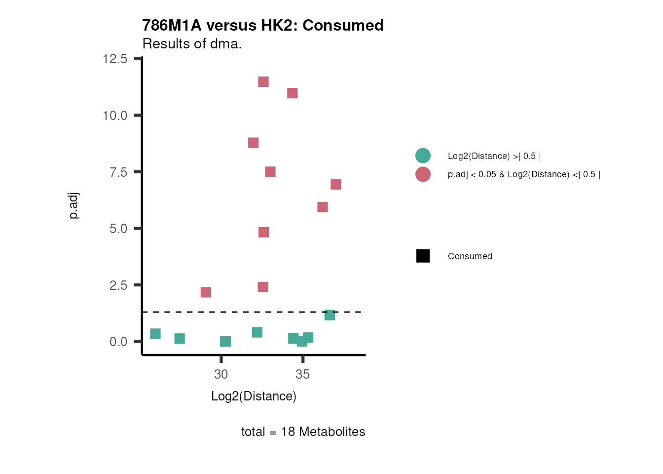

Standard figure displaying dma results.

#> Warning: Removed 2 rows containing missing values or values outside the scale range
#> (`geom_vline()`).
#> Removed 2 rows containing missing values or values outside the scale range
#> (`geom_vline()`).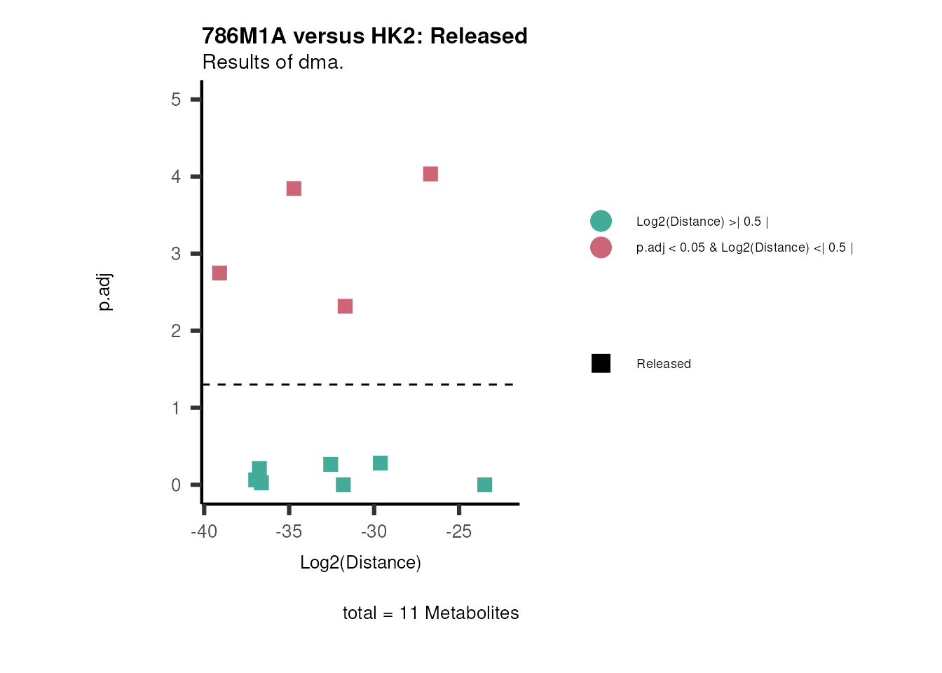

Standard figure displaying dma results.

Given that we also know, which metabolic pathway the metabolites correspond to, we can add this information into the plot. This is also a good example to showcase the flexibility of the visualisation function: Either you use the parameter metadata_feature = MetaData_Metab as above, but as we have the column “Pathway” also in our data you can also pass metadata_feature = DMA_HK2_vs_786M1A or simply use the default metadata_feature = NULL, in which case the metadata_info information (here color) will be used from data.

# Now we can use color for the pathways and shape for the metabolite clusters:
viz_volcano(plot_types="Standard",
metadata_info= c(individual="core", shape="core_specific", color="Pathway"),
metadata_feature= MetaData_Metab,
data=DMA_HK2_vs_786M1A%>%column_to_rownames("Metabolite"),
x= "Log2(Distance)",
plot_name= "786M1A versus HK2",
subtitle= "Results of dma." )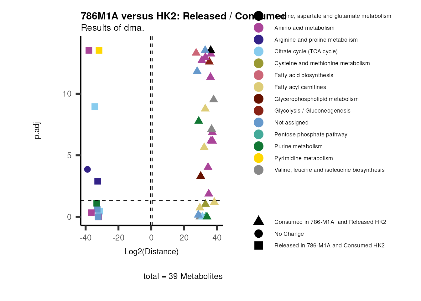

Standard figure displaying dma results colour coded for metabolic pathways and shaped for metabolic clusters.

#> Warning: Removed 2 rows containing missing values or values outside the scale range
#> (`geom_vline()`).
#> Removed 2 rows containing missing values or values outside the scale range
#> (`geom_vline()`).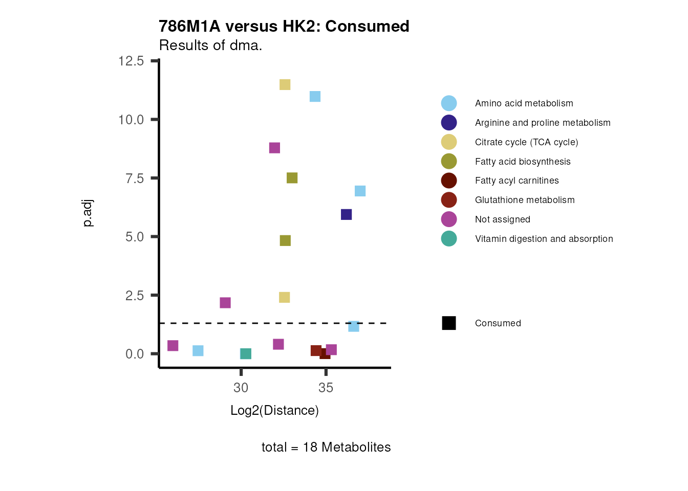

Standard figure displaying dma results colour coded for metabolic pathways and shaped for metabolic clusters.

#> Warning: Removed 2 rows containing missing values or values outside the scale range
#> (`geom_vline()`).
#> Removed 2 rows containing missing values or values outside the scale range
#> (`geom_vline()`).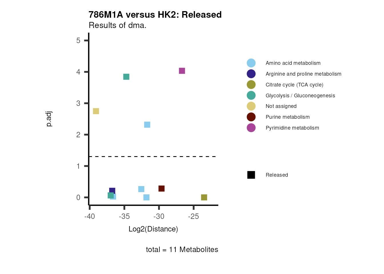

Standard figure displaying dma results colour coded for metabolic pathways and shaped for metabolic clusters.

Comparison

The parameter plot_types = "Compare" is helpful if you have performed multiple comparisons and seek to compare two of them in one plot:

# Make the plot
viz_volcano(plot_types="Compare",
data=DMA_HK2_vs_786M1A%>%column_to_rownames("Metabolite"),
data2= DMA_Annova[["dma"]][["HK2_vs_786-O"]]%>%column_to_rownames("Metabolite"),
name_comparison= c(data="HK2_vs_786-M1A", data2= "HK2_vs_786-O"),
x= "Log2(Distance)",
plot_name= "786M1A vs HK2 compared to 7860 vs HK2",
subtitle= "Results of dma" )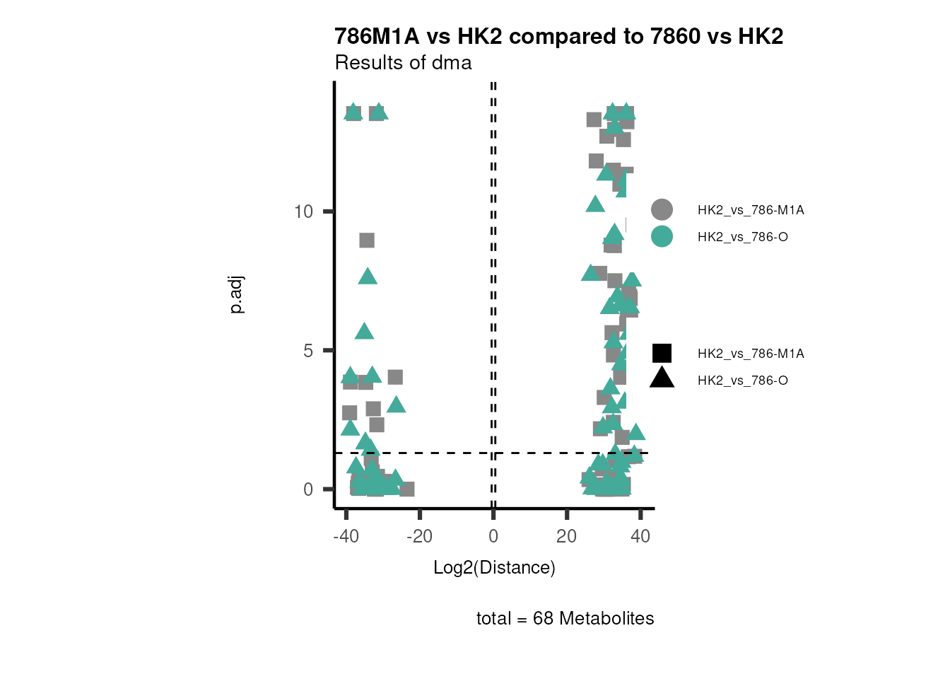

Comparison.

Of course you have option to use shape or color to further customize your graph as well as make individual plots:

# Make the plot
viz_volcano(plot_types="Compare",
metadata_info= c(color="Pathway"),
metadata_feature= MetaData_Metab,
data=DMA_HK2_vs_786M1A%>%column_to_rownames("Metabolite"),
data2= DMA_Annova[["dma"]][["HK2_vs_786-O"]]%>%column_to_rownames("Metabolite"),
name_comparison= c(data="HK2_vs_786-M1A", data2= "HK2_vs_786-O"),
x= "Log2(Distance)",
plot_name= "786M1A vs HK2 compared to 7860 vs HK2",
subtitle= "Results of dma" )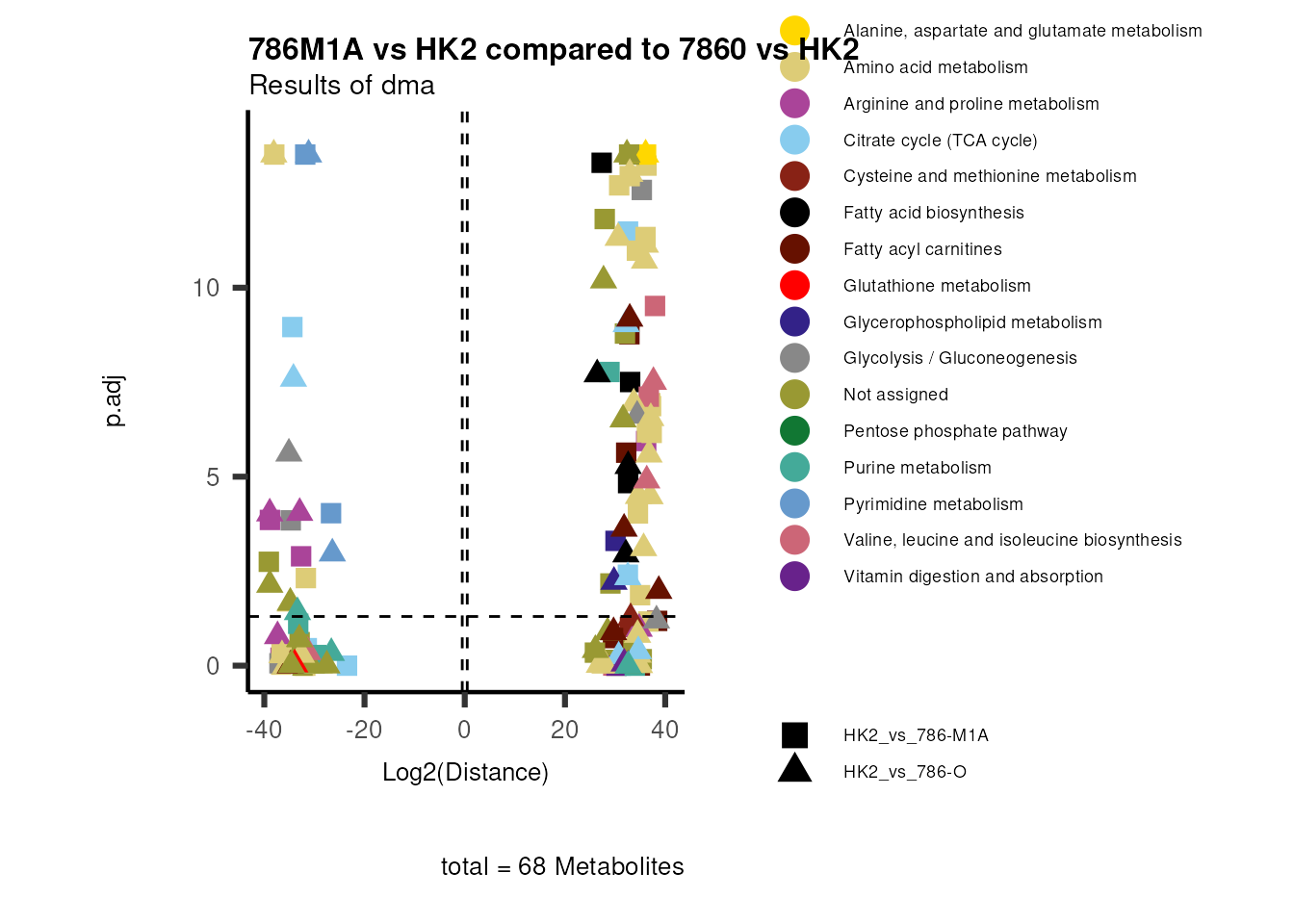

Comparison.

Now we do individual plots again:

viz_volcano(plot_types="Compare",
metadata_info= c(individual="Pathway"),
metadata_feature= MetaData_Metab,
data=DMA_HK2_vs_786M1A%>%column_to_rownames("Metabolite"),
data2= DMA_Annova[["dma"]][["HK2_vs_786-O"]]%>%column_to_rownames("Metabolite"),
name_comparison= c(data="HK2_vs_786-M1A", data2= "HK2_vs_786-O"),
x= "Log2(Distance)",
plot_name= "786M1A vs HK2 compared to 7860 vs HK2",
subtitle= "Results of dma" )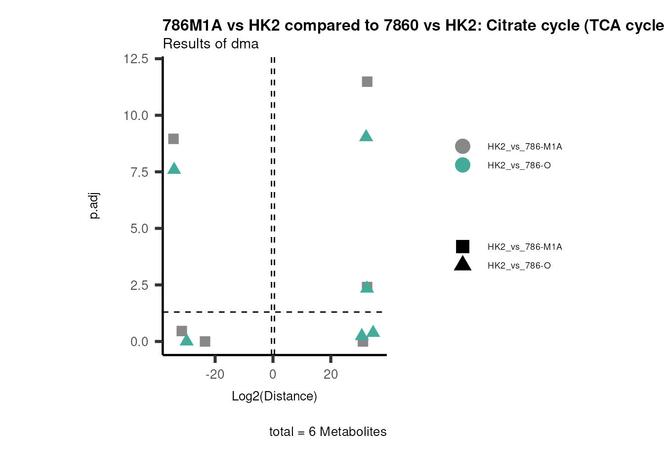

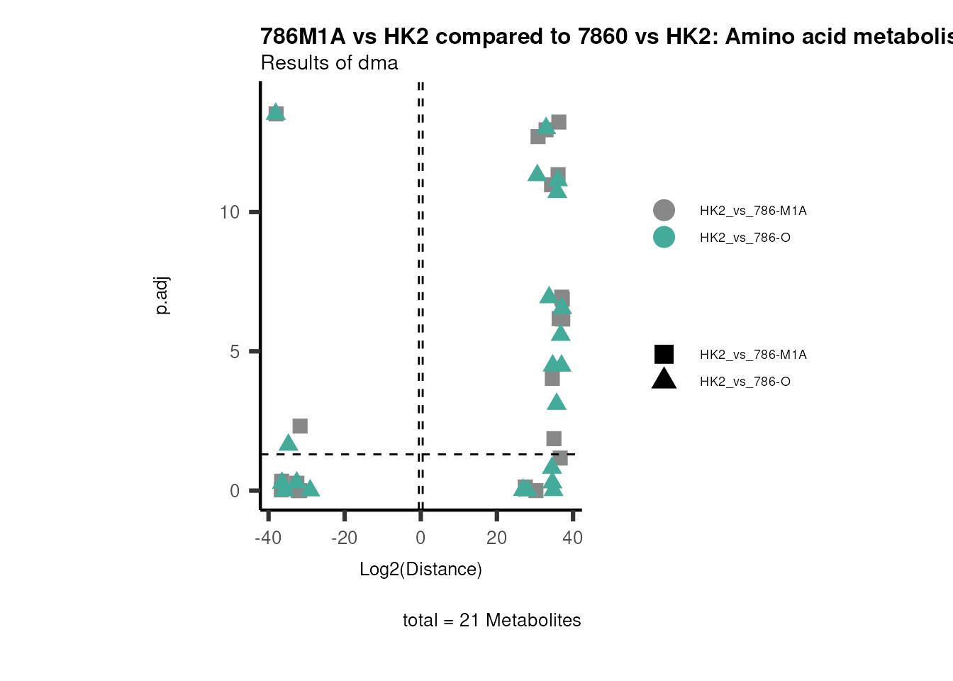
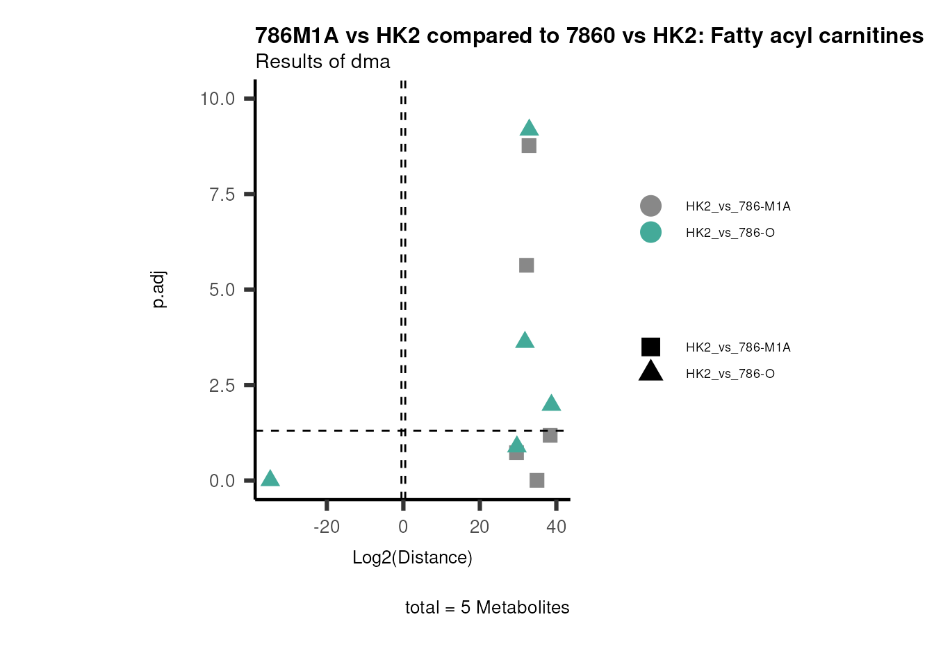
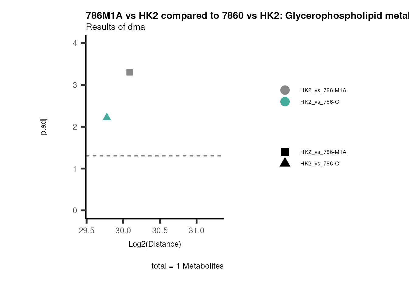
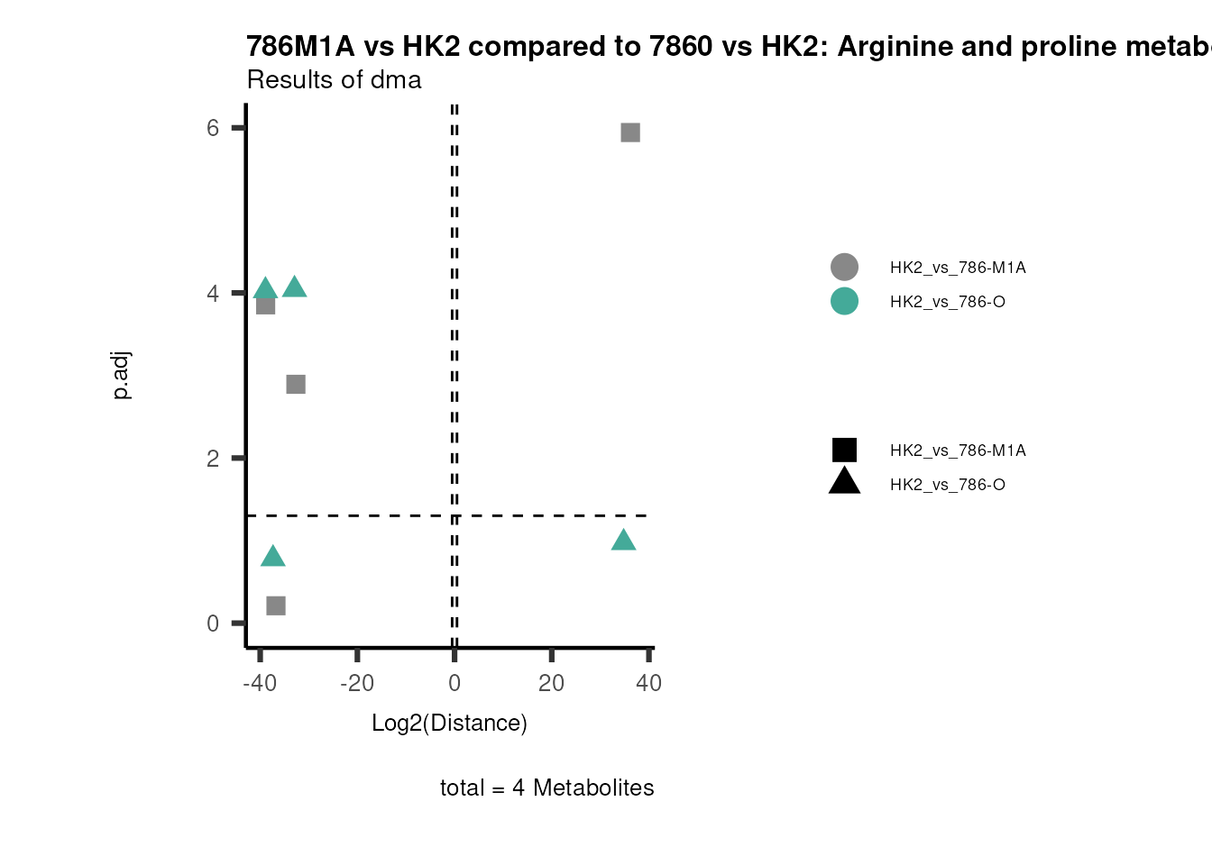
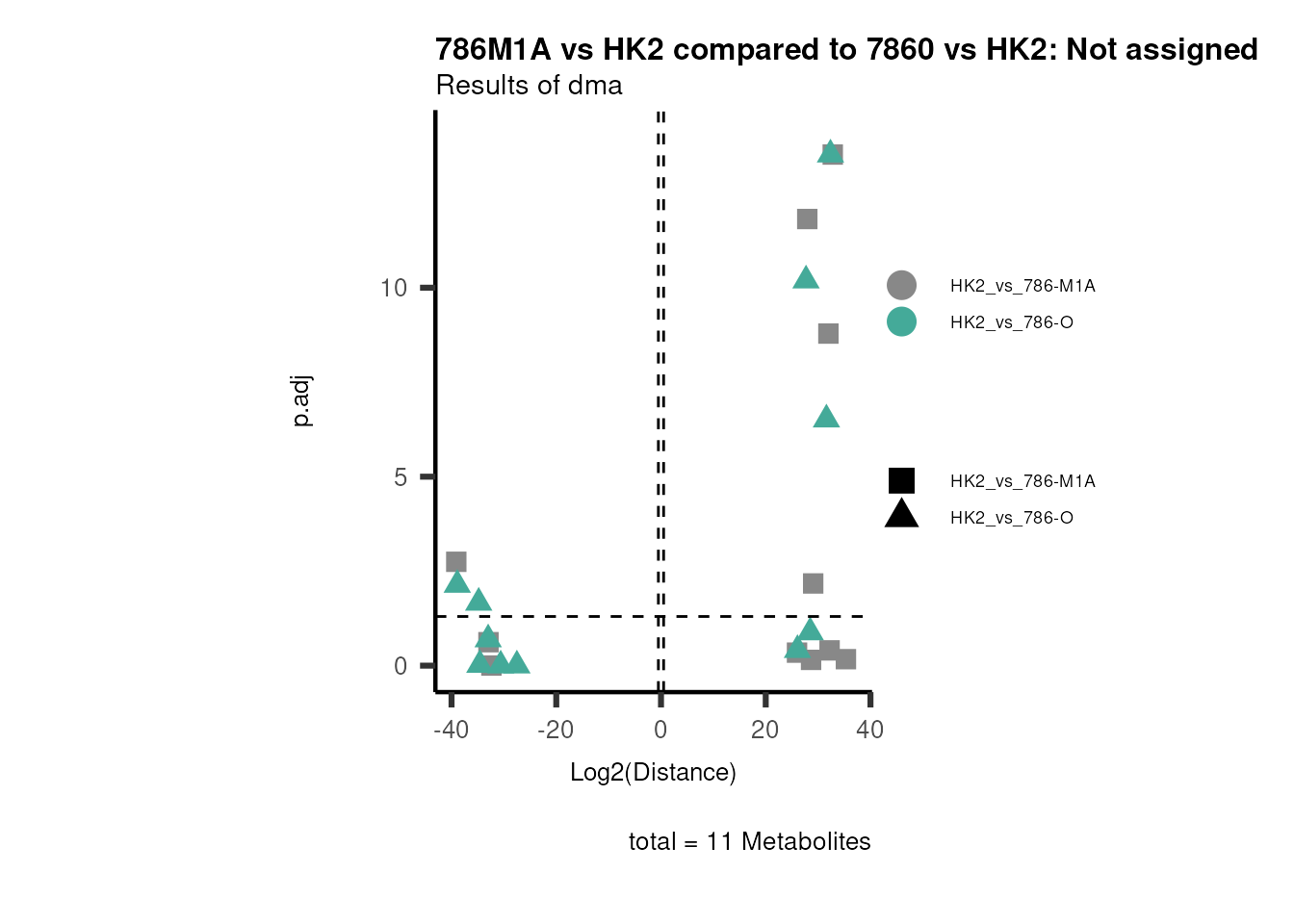
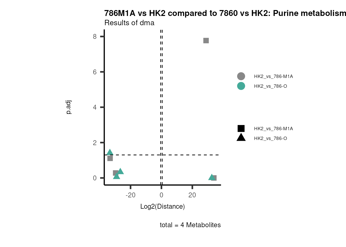
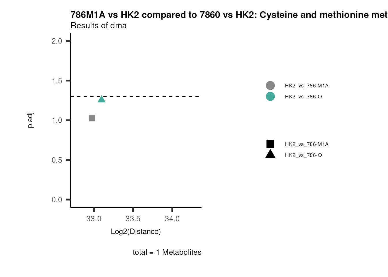
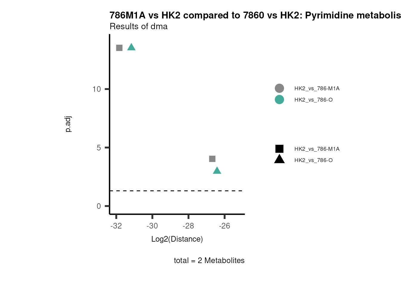
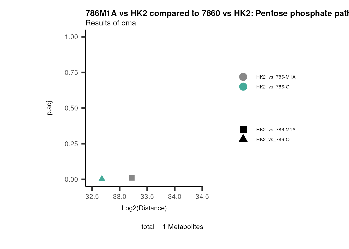
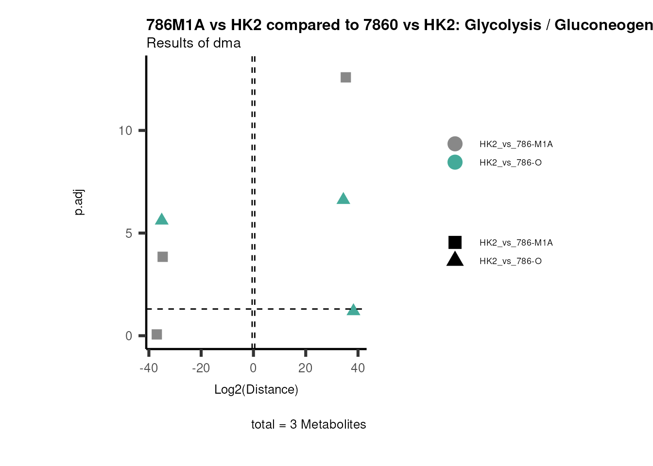
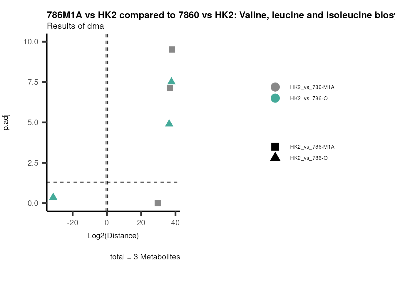
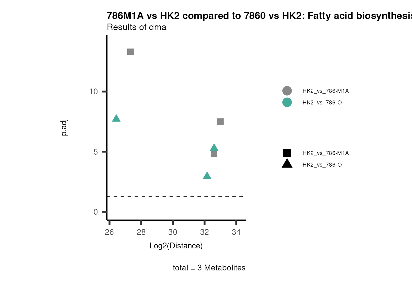
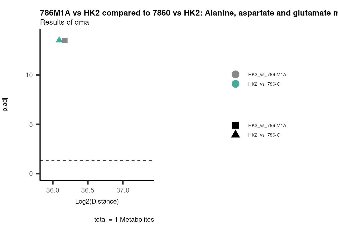
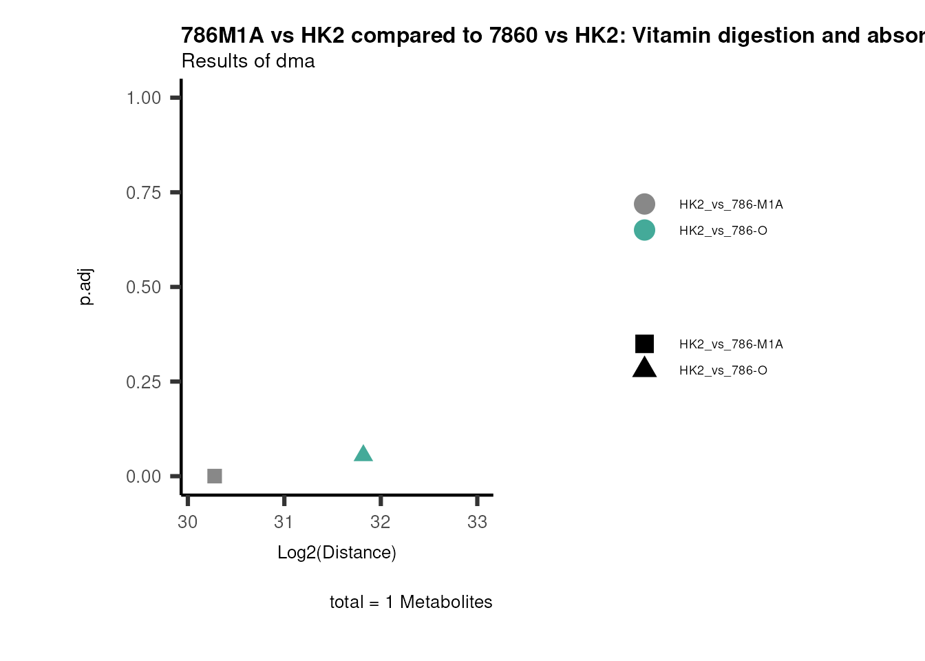
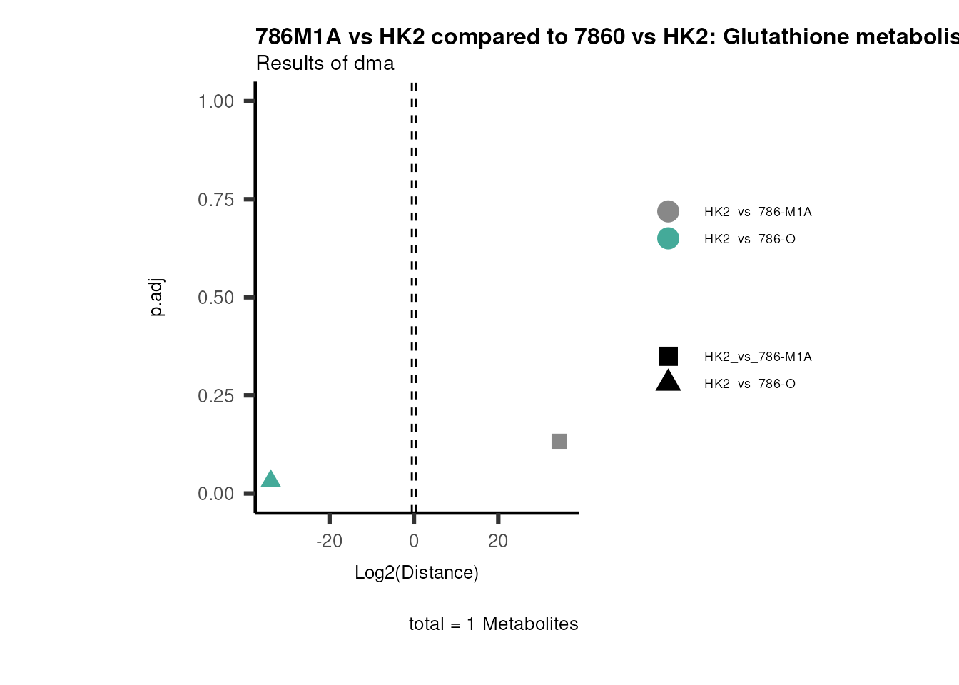
PathwayEnrichmentAnalysis

If you have performed Pathway Enrichment Analysis (PEA) such as ORA or GSEA, we can also plot the results and add the information into the Figure legends.
Here we can for example use the results of the ORA we have performed on the differential expression results. Indeed for DMA_HK2_vs_786M1A we have performed ORA on each cluster (consumed, released, consumed/released). Here, I will plot the ORA results of the metabolites that are consumed in both conditions, HK2 and 786-M1A. As one plot is made for each pathway, we only use the 10 pathways with the lowest adjusted p-value.

# Prepare the Input:
# 1. data=Pathway analysis input: Must have features as column names. Those feature names need to match features in the pathway analysis file metadata_feature.
InputPEA <- DMA_HK2_vs_786M1A %>%
filter(!is.na(KEGGCompound)) %>%
column_to_rownames("KEGGCompound")

# 2. data2=Pathway analysis output: Must have same column names as metadata_feature for Pathway name
InputPEA2 <- MC_ORA_HK2_vs_786M1A_Consumed %>%
dplyr::rename("term"="ID") %>%
dplyr::slice_min(p.adjust, n = 10, with_ties = FALSE) # top 10 pathways

# 3. metadata_feature= Pathways used for pathway analysis: Must have same column names as metadata_feature for Pathway name and feature names need to match features in the data. PEA_Feature passes this column name!

viz_volcano(plot_types="PEA",
metadata_info= c(PEA_Pathway="term",# Needs to be the same in both, metadata_feature and data2.
PEA_stat="p.adjust",#Column data2
PEA_score="GeneRatio",#Column data2
PEA_Feature="Metabolite"),# Column metadata_feature (needs to be the same as row names in data)
metadata_feature= KEGG_Pathways,#Must be the pathways used for pathway analysis
data= InputPEA, #Must be the data you have used as an input for the pathway analysis
data2= InputPEA2, #Must be the results of the pathway analysis
x= "Log2(Distance)",
plot_name= "KEGG",
subtitle= "PEA" ,
select_label = NULL)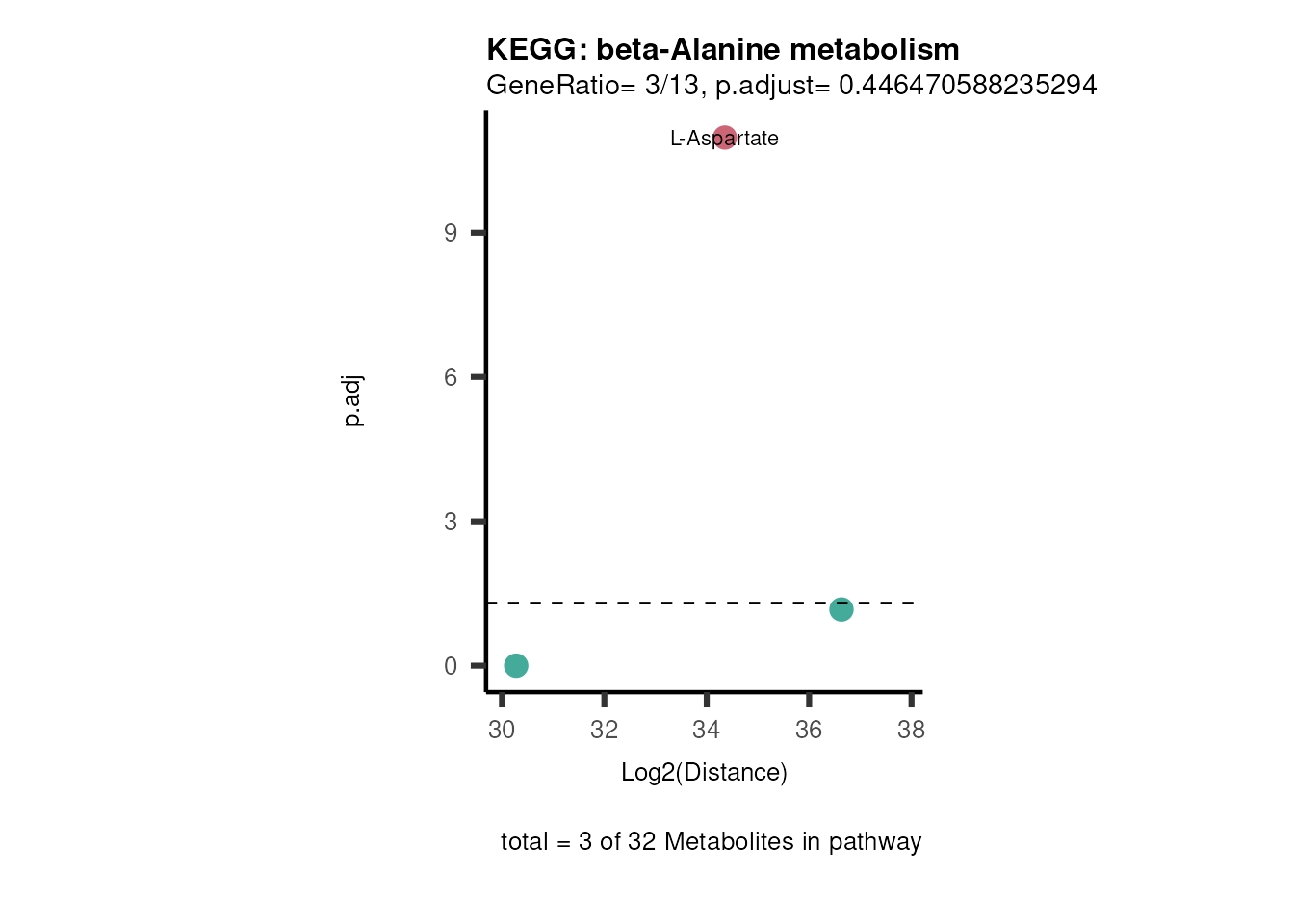

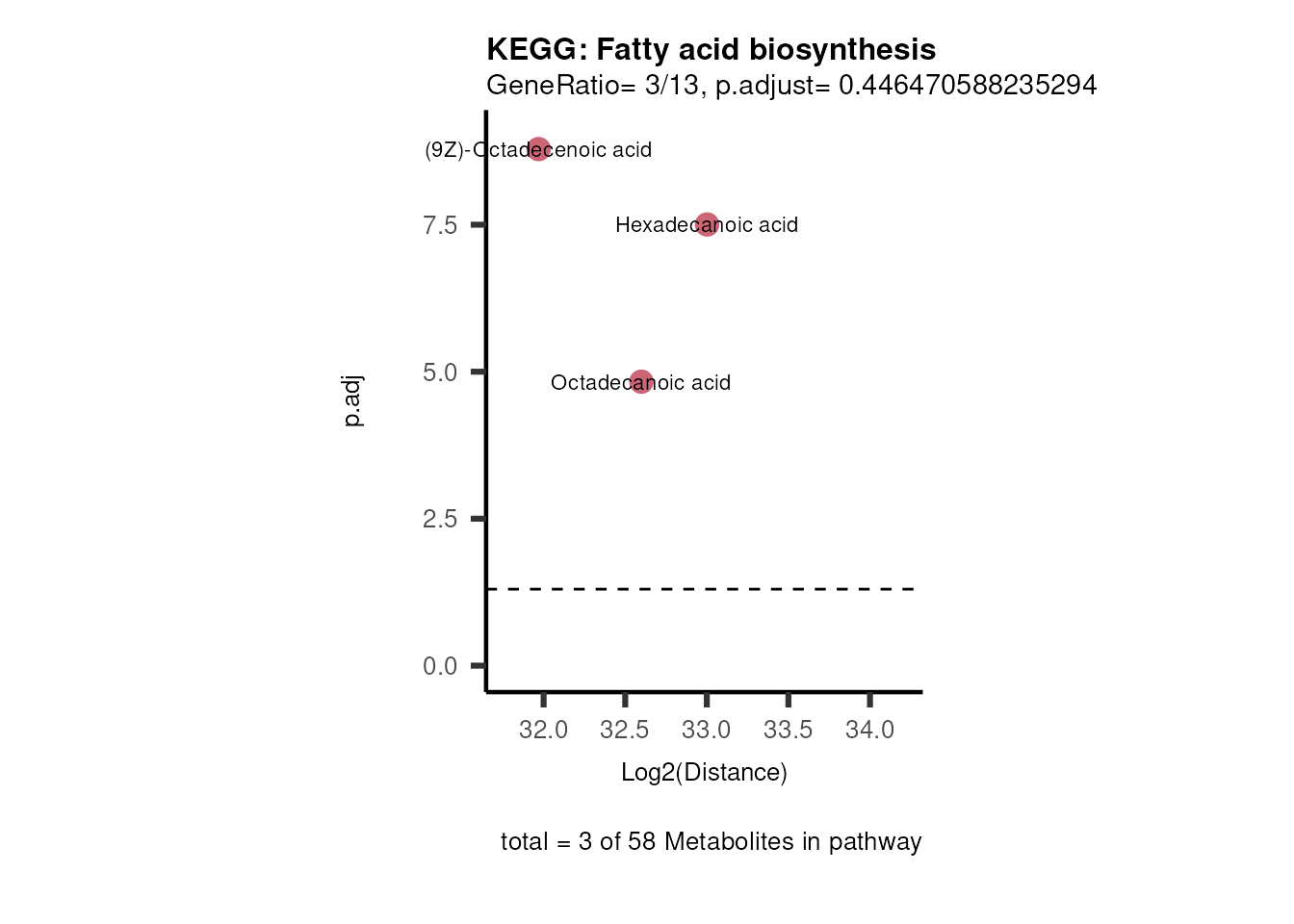
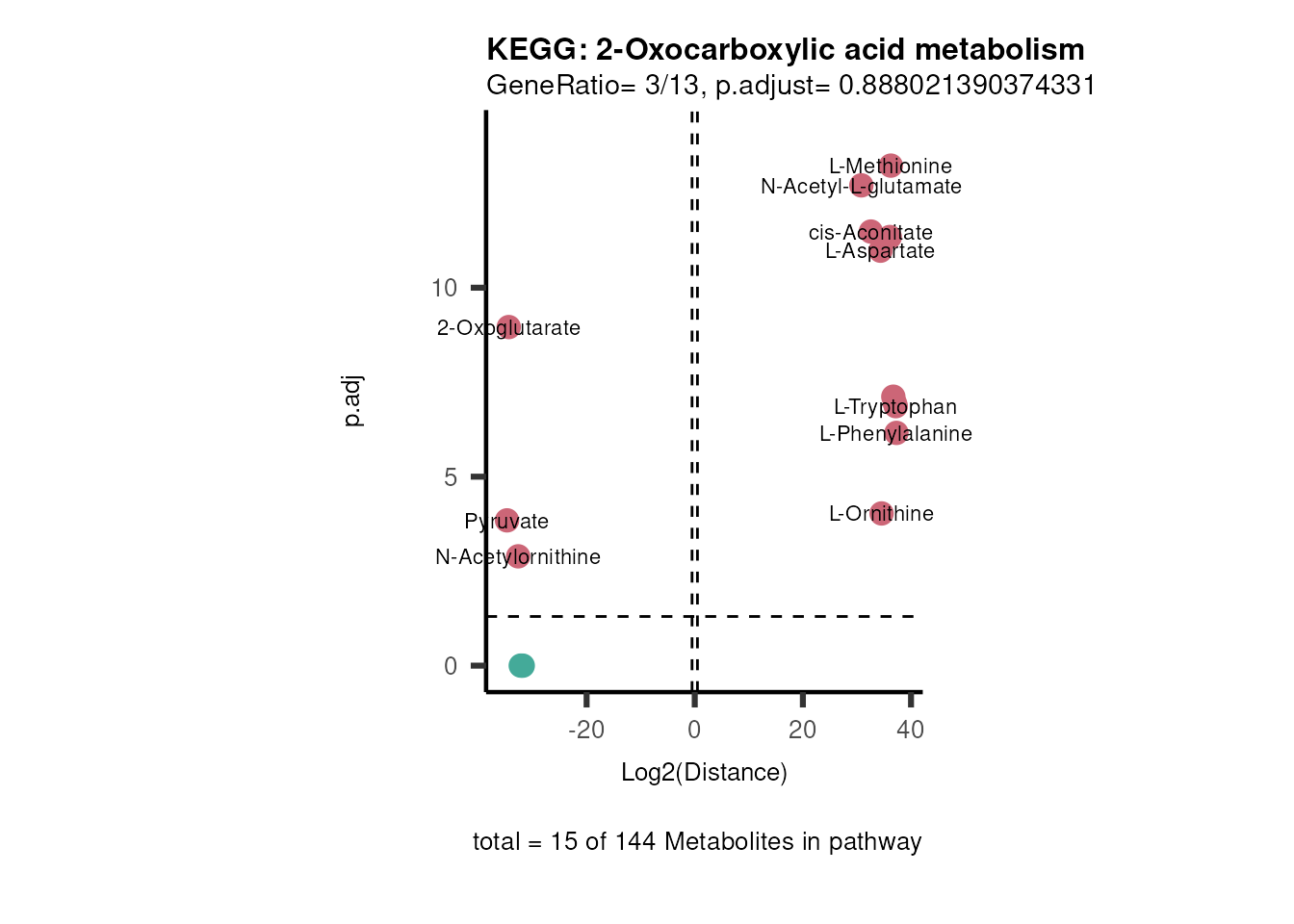
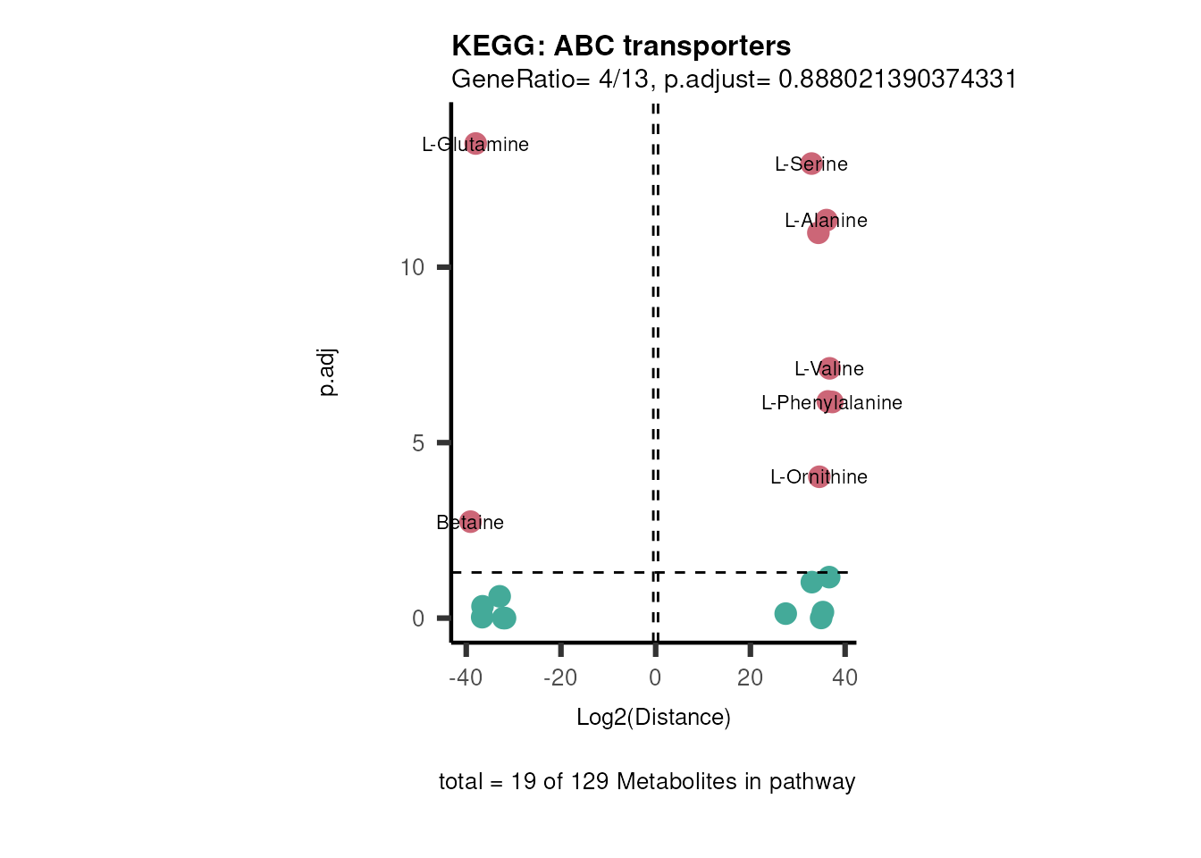
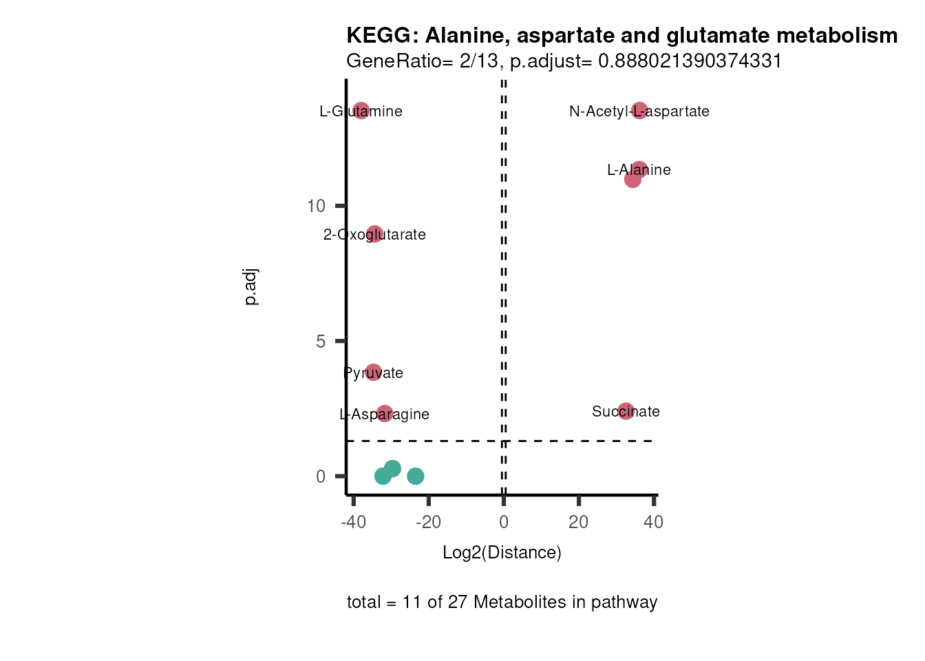
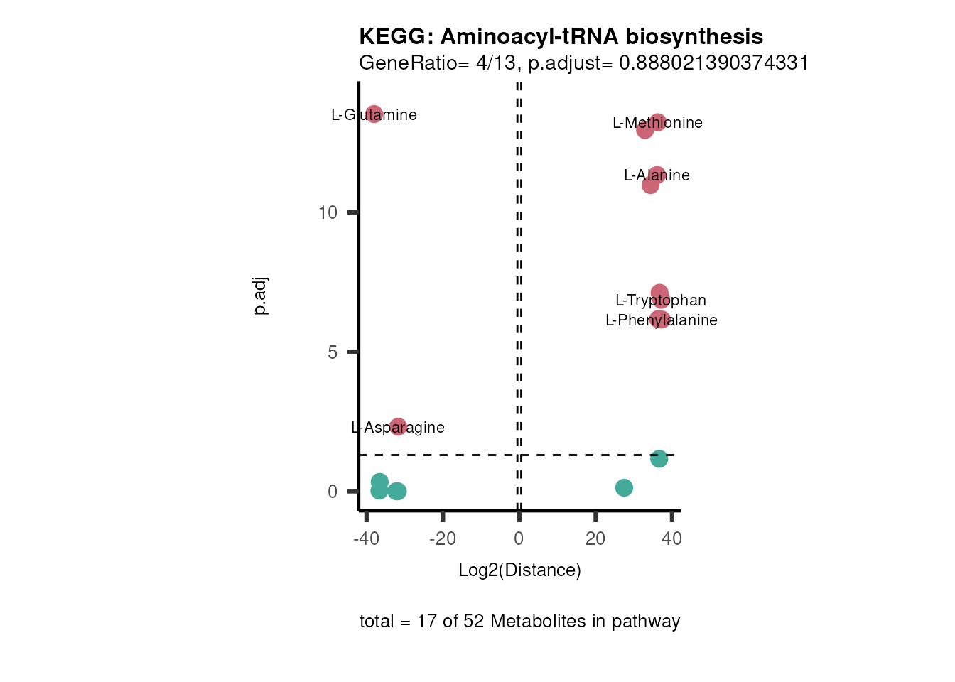
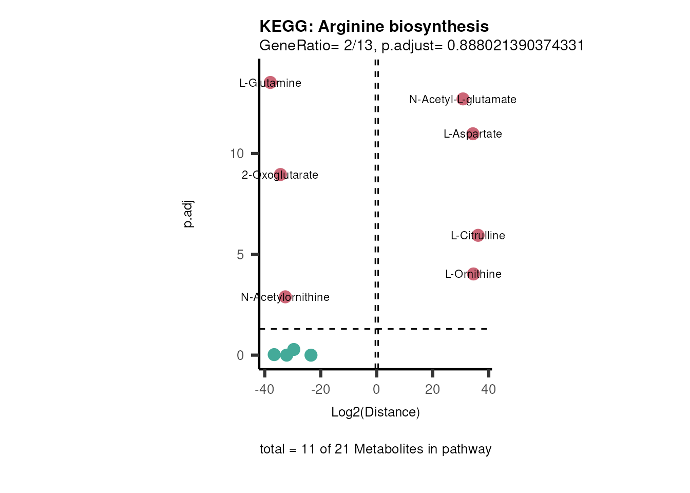
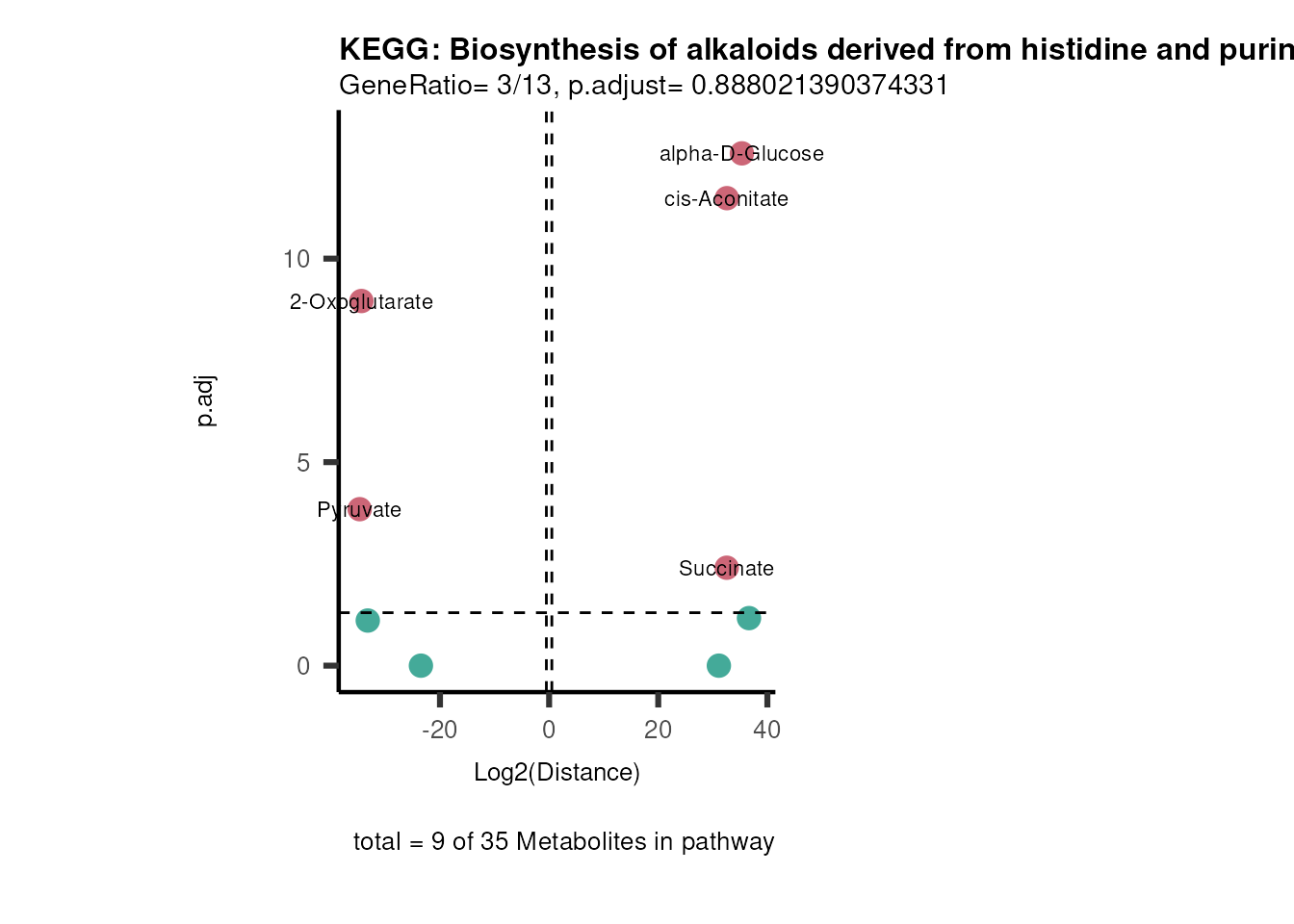
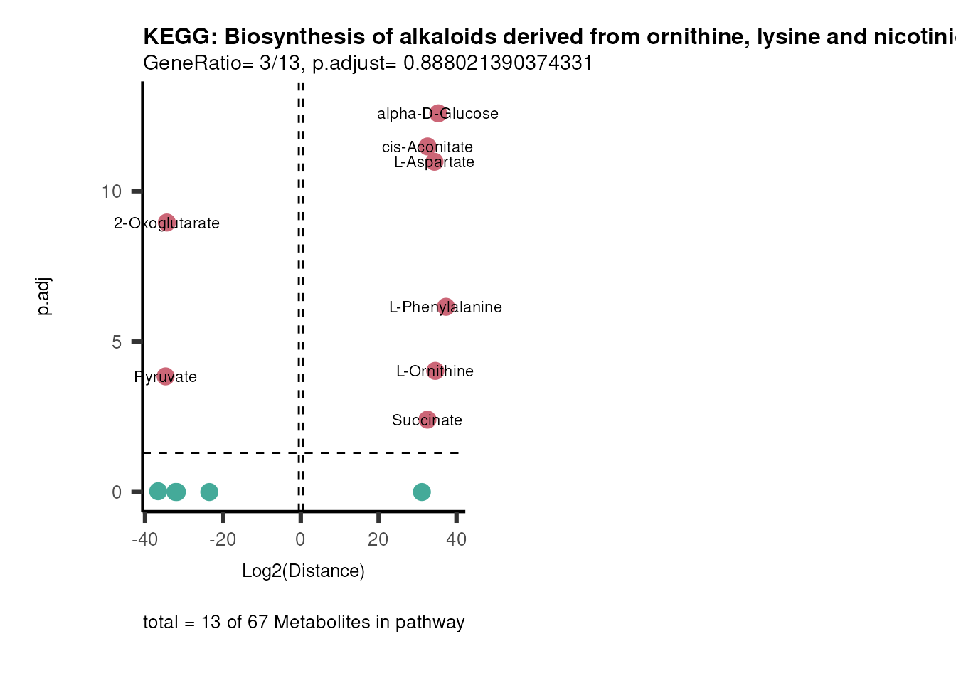
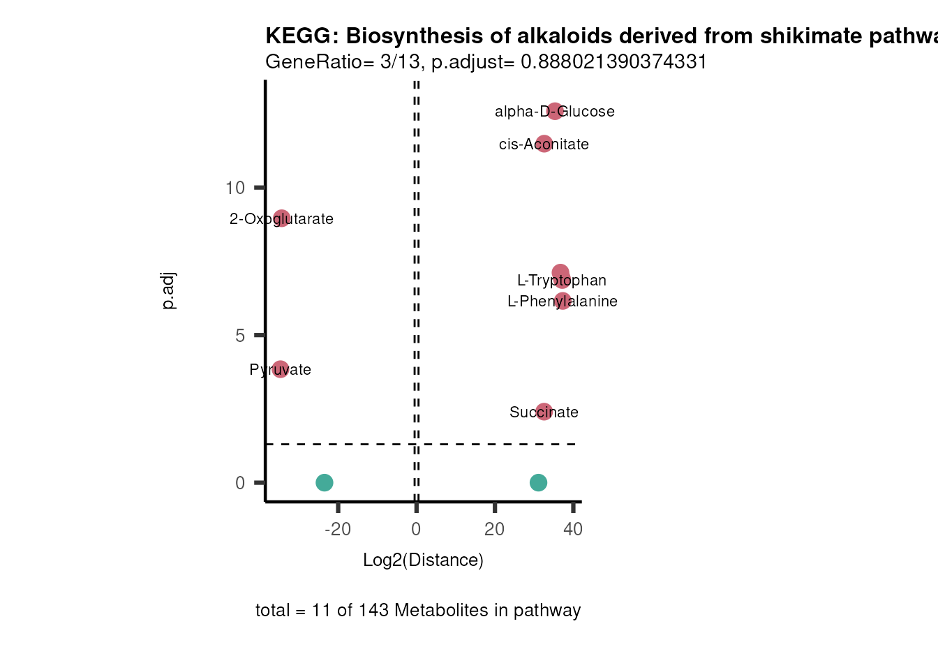
Session information

#> R version 4.6.1 (2026-06-24)
#> Platform: x86_64-pc-linux-gnu
#> Running under: Ubuntu 24.04.4 LTS
#> 
#> Matrix products: default
#> BLAS:   /usr/lib/x86_64-linux-gnu/openblas-pthread/libblas.so.3 
#> LAPACK: /usr/lib/x86_64-linux-gnu/openblas-pthread/libopenblasp-r0.3.26.so;  LAPACK version 3.12.0
#> 
#> locale:
#>  [1] LC_CTYPE=en_US.UTF-8       LC_NUMERIC=C               LC_TIME=en_US.UTF-8        LC_COLLATE=en_US.UTF-8    
#>  [5] LC_MONETARY=en_US.UTF-8    LC_MESSAGES=en_US.UTF-8    LC_PAPER=en_US.UTF-8       LC_NAME=C                 
#>  [9] LC_ADDRESS=C               LC_TELEPHONE=C             LC_MEASUREMENT=en_US.UTF-8 LC_IDENTIFICATION=C       
#> 
#> time zone: Etc/UTC
#> tzcode source: system (glibc)
#> 
#> attached base packages:
#> [1] stats     graphics  grDevices utils     datasets  methods   base     
#> 
#> other attached packages:
#> [1] stringr_1.6.0     ggfortify_0.4.24  ggplot2_4.0.3     rlang_1.3.0       tibble_3.3.1      dplyr_1.2.1      
#> [7] magrittr_2.0.5    MetaProViz_4.99.0 BiocStyle_2.40.0 
#> 
#> loaded via a namespace (and not attached):
#>   [1] RColorBrewer_1.1-3          rstudioapi_0.19.0           jsonlite_2.0.0              magick_2.9.1               
#>   [5] ggbeeswarm_0.7.3            farver_2.1.2                rmarkdown_2.32              fs_2.1.0                   
#>   [9] ragg_1.5.2                  vctrs_0.7.3                 memoise_2.0.1               tinytex_0.61               
#>  [13] rstatix_1.1.0               htmltools_0.5.9             S4Arrays_1.12.1             progress_1.2.3             
#>  [17] curl_8.0.0                  ComplexUpset_1.3.3          decoupleR_2.17.0            broom_1.0.13               
#>  [21] cellranger_1.1.0            SparseArray_1.12.3          Formula_1.2-6               sass_0.4.10                
#>  [25] parallelly_1.48.0           bslib_0.12.0                htmlwidgets_1.6.4           desc_1.4.3                 
#>  [29] plyr_1.8.9                  httr2_1.3.0                 lubridate_1.9.5             cachem_1.1.0               
#>  [33] igraph_2.3.4                lifecycle_1.0.5             pkgconfig_2.0.3             Matrix_1.7-6               
#>  [37] R6_2.6.1                    fastmap_1.2.0               MatrixGenerics_1.24.0       digest_0.6.39              
#>  [41] colorspace_2.1-3            patchwork_1.3.2             S4Vectors_0.50.3            textshaping_1.0.5          
#>  [45] GenomicRanges_1.64.0        RSQLite_3.53.3              ggpubr_1.0.0                labeling_0.4.3             
#>  [49] timechange_0.4.0            polyclip_1.10-7             httr_1.4.9                  abind_1.4-8                
#>  [53] compiler_4.6.1              bit64_4.8.6                 withr_3.0.3                 S7_0.2.2                   
#>  [57] backports_1.5.1             BiocParallel_1.46.0         viridis_0.6.5               carData_3.0-6              
#>  [61] DBI_1.3.0                   logger_0.4.3                OmnipathR_4.1.0             ggforce_0.5.0              
#>  [65] R.utils_2.13.0              ggsignif_0.6.4              cosmosR_1.20.0              MASS_7.3-66                
#>  [69] rappdirs_0.3.4              DelayedArray_0.38.2         sessioninfo_1.2.4           scatterplot3d_0.3-45       
#>  [73] gtools_3.9.5                tools_4.6.1                 vipor_0.4.7                 otel_0.2.0                 
#>  [77] beeswarm_0.4.0              zip_3.0.2                   R.oo_1.27.1                 glue_1.8.1                 
#>  [81] grid_4.6.1                  checkmate_2.3.4             reshape2_1.4.5              generics_0.1.4             
#>  [85] gtable_0.3.6                tzdb_0.5.0                  R.methodsS3_1.8.2           tidyr_1.3.2                
#>  [89] hms_1.1.4                   tidygraph_1.3.1             xml2_1.6.0                  car_3.1-5                  
#>  [93] XVector_0.52.0              BiocGenerics_0.58.1         ggrepel_0.9.8               pillar_1.11.1              
#>  [97] vroom_1.7.1                 limma_3.68.5                later_1.4.8                 splines_4.6.1              
#> [101] tweenr_2.0.3                lattice_0.22-9              bit_4.6.0                   tidyselect_1.2.1           
#> [105] knitr_1.52                  gridExtra_2.3.1             bookdown_0.48               IRanges_2.46.0             
#> [109] Seqinfo_1.2.0               SummarizedExperiment_1.42.0 svglite_2.2.2               stats4_4.6.1               
#> [113] xfun_0.61                   graphlayouts_1.2.5          Biobase_2.72.0              statmod_1.5.2              
#> [117] factoextra_2.2.0            matrixStats_1.5.0           pheatmap_1.0.13             stringi_1.8.9              
#> [121] yaml_2.3.12                 kableExtra_1.4.1            evaluate_1.0.5              codetools_0.2-20           
#> [125] tcltk_4.6.1                 ggraph_2.2.2                qvalue_2.44.0               hash_2.2.6.4               
#> [129] BiocManager_1.30.27         Polychrome_1.6.2            cli_3.6.6                   systemfonts_1.3.2          
#> [133] jquerylib_0.1.4             EnhancedVolcano_1.31.0      Rcpp_1.1.2                  readxl_1.5.0.1             
#> [137] XML_3.99-0.25               parallel_4.6.1              pkgdown_2.2.1               readr_2.2.0                
#> [141] blob_1.3.0                  prettyunits_1.2.0           viridisLite_0.4.3           scales_1.4.0               
#> [145] writexl_2.0.1               inflection_1.3.7            purrr_1.2.2                 crayon_1.5.3               
#> [149] rvest_1.0.5

Badia-I-Mompel, Pau, Jesús Vélez Santiago, Jana Braunger, et al. 2022. “decoupleR: Ensemble of Computational Methods to Infer Biological Activities from Omics Data.” Bioinformatics Advances 2 (1): vbac016. https://doi.org/10.1093/bioadv/vbac016.

Bijlsma, Sabina, Ivana Bobeldijk, Elwin R Verheij, et al. 2006. “Large-Scale Human Metabolomics Studies: A Strategy for Data (Pre-) Processing and Validation.” Analytical Chemistry 78 (2): 567–74. https://doi.org/10.1021/ac051495j.

Farr, Elias, Daniel Dimitrov, Christina Schmidt, et al. 2024. “MetalinksDB: A Flexible and Contextualizable Resource of Metabolite-Protein Interactions.” Briefings in Bioinformatics, no. 4 (May). https://doi.org/10.1093/bib/bbae347.

Hotelling, Harold. 1931. “The Generalization of Student’s Ratio.” The Annals of Mathematical Statistics 2 (3): 360–78. https://doi.org/10.1214/aoms/1177732979.

Kanehisa, M, and S Goto. 2000. “KEGG: Kyoto Encyclopedia of Genes and Genomes.” Nucleic Acids Research 28 (1): 27–30. https://doi.org/10.1093/nar/28.1.27.

Lord, Samuel J, Katrina B Velle, R Dyche Mullins, and Lillian K Fritz-Laylin. 2020. “SuperPlots: Communicating Reproducibility and Variability in Cell Biology.” The Journal of Cell Biology, no. 6 (June). https://doi.org/10.1083/jcb.202001064.

Wei, Runmin, Jingye Wang, Mingming Su, et al. 2018. “Missing Value Imputation Approach for Mass Spectrometry-Based Metabolomics Data.” Scientific Reports 8 (1): 663. https://doi.org/10.1038/s41598-017-19120-0.

Wulff, Jacob E., and Matthew W. Mitchell. 2018. “A Comparison of Various Normalization Methods for LC/MS Metabolomics Data.” Advances in Bioscience and Biotechnology 09 (08): 339–51. https://doi.org/10.4236/abb.2018.98022.