Sample Metadata Analysis

Tissue metabolomics experiment is a standard metabolomics experiment using tissue samples (e.g. from animals or patients).

In this tutorial we showcase how to use MetaProViz:

to perform differential metabolite analysis (dma) to generate Log2FC and statistics and perform pathway analysis using Over Representation Analysis (ORA) on the results.
to do metabolite clustering analysis (MCA) to find clusters of metabolites with similar behaviors based on patients demographics like age, gender and tumour stage.
Find the main metabolite drivers that separate patients based on their demographics like age, gender and tumour stage.

First if you have not done yet, install the required dependencies and load the libraries:

# 1. Install MetaProViz from Bioconductor devel:
# if (!requireNamespace("BiocManager", quietly = TRUE)) install.packages("BiocManager")
# BiocManager::install(version = "devel")
# BiocManager::install("MetaProViz")
# 2. Install the latest development version from GitHub using devtools
# remotes::install_github("saezlab/MetaProViz") # Install Rtools if you haven’t done this yet, using the appropriate version (e.g.windows or macOS).

library(MetaProViz)

# dependencies that need to be loaded:
library(magrittr)
library(dplyr)
library(rlang)
library(tidyr)
library(tibble)
library(stringr)

Loading the example data

Here we choose an example dataset, which is publicly available in the paper “An Integrated Metabolic Atlas of Clear Cell Renal Cell Carcinoma”, which includes metabolomic profiling on 138 matched clear cell renal cell carcinoma (ccRCC)/normal tissue pairs (Hakimi et al. 2016). Metabolomics was done using the company Metabolon, so this is untargeted metabolomics. Here we use the median normalised data from the supplementary table 2 of the paper. We have combined the metainformation about the patients with the metabolite measurements and removed unidentified metabolites. Lastly, we have added a column “Stage” where Stage1 and Stage2 patients are summarised to “EARLY-STAGE” and Stage3 and Stage4 patients to “LATE-STAGE”. Moreover, we have added a column “Age”, where patients with “AGE AT SURGERY” <42 are defined as “Young” and patients with AGE AT SURGERY >58 as “Old” and the remaining patients as “Middle”.

As part of the MetaProViz package you can load the example data into your global environment using data():
1. Tissue experiment (Intra)
We can access the built-in dataset tissue_norm, which includes columns with Sample information and columns with the median normalised measured metabolite integrated peaks.

# Load the example data:
data(tissue_norm)

Tissue_Norm <- tissue_norm%>%
column_to_rownames("Code")

Preview of the DF `Tissue_Norm` including columns with sample information and metabolite ids with their measured values.
	TISSUE_TYPE	GENDER	AGE_AT_SURGERY	TYPE-STAGE	STAGE	AGE	1,2-propanediol	1,3-dihydroxyacetone
DIAG-16076	TUMOR	Male	74.7778	TUMOR-STAGE I	EARLY-STAGE	Old	0.710920	0.809182
DIAG-16077	NORMAL	Male	74.7778	NORMAL-STAGE I	EARLY-STAGE	Old	0.339390	0.718725
DIAG-16078	TUMOR	Male	77.1778	TUMOR-STAGE I	EARLY-STAGE	Old	0.413386	0.276412
DIAG-16079	NORMAL	Male	77.1778	NORMAL-STAGE I	EARLY-STAGE	Old	1.595697	4.332451
DIAG-16080	TUMOR	Female	59.0889	TUMOR-STAGE I	EARLY-STAGE	Old	0.573787	0.646791

2. Additional information mapping the trivial metabolite names to KEGG IDs, HMDB IDs, etc. and selected pathways (MappingInfo)

data(tissue_meta)

Tissue_MetaData <- tissue_meta%>%
    dplyr::filter(!stringr::str_detect(Metabolite, "^X\\s*-\\s*\\d+$"))# remove rows without identification

Preview of the DF `Tissue_MetaData` including the trivial metabolite identifiers used in the experiment as well as IDs and pathway information.
Metabolite	CAS	RI	MASS	PUBCHEM	KEGG
1,2-propanediol	57-55-6;	1041	117	NA	C00583
1,3-dihydroxyacetone	62147-49-3;	1263	103	670	C00184
1,5-anhydroglucitol (1,5-AG)	154-58-5;	1788.7	217	NA	C07326
1-arachidonoylglycerophosphocholine*	NA	5554	544.29999999999995	NA	C05208
1-arachidonoylglycerophosphoethanolamine*	NA	5731	500.3	NA	NA

Run MetaProViz Analysis

Pre-processing

This has been done by the authors of the paper and we will use the median normalized data. If you want to know how you can use the MetaProViz pre-processing module, please check out the vignette:
- Standard metabolomics data
- Consumption-Release (core) metabolomics data from cell culture media

Metadata analysis

We can use the patient’s metadata to find the main metabolite drivers that separate patients based on their demographics like age, gender, etc.

Here the metadata analysis is based on principal component analysis (PCA), which is a dimensionality reduction method that reduces all the measured features (=metabolites) of one sample into a few features in the different principal components, whereby each principal component can explain a certain percentage of the variance between the different samples. Hence, this enables interpretation of sample clustering based on the measured features (=metabolites).
The metadata_analysis() function will perform PCA to extract the different PCs followed by ANOVA to find the main metabolite drivers that separate patients based on their demographics.

MetaRes <- metadata_analysis(data=Tissue_Norm[,-c(1:13)],
metadata_sample= Tissue_Norm[,c(2,4:5,12:13)],
scaling = TRUE,
percentage = 0.1,
cutoff_stat= 0.05,
cutoff_variance = 1)
#> The column names of the 'metadata_sample' contain special character that where removed.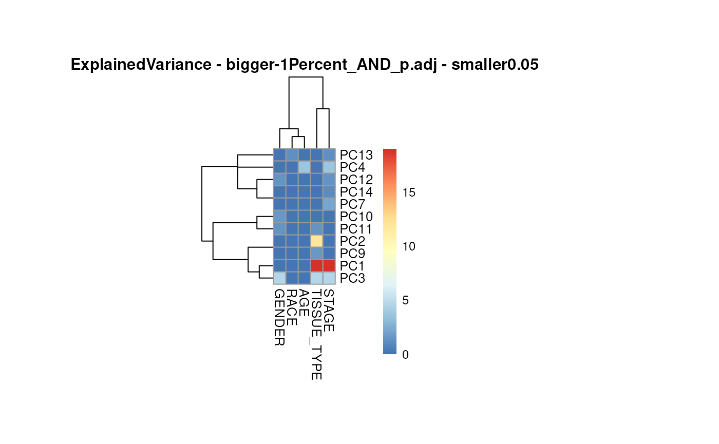

Ultimately, this is leading to clusters of metabolites that are driving the separation of the different demographics.

We generated the general anova output DF:

Preview of the DF MetaRes[[`res_aov`]] including the main metabolite drivers that separate patients based on their demographics.
	PC	tukeyHSD_Contrast	term	anova_sumsq	anova_meansq	anova_statistic	anova_p.value	tukeyHSD_p.adjusted	Explained_Variance
1	PC1	TUMOR-NORMAL	TISSUE_TYPE	7375.2212254	7375.2212254	90.1352800	0.0000000	0.0000000	19.0079573
2	PC1	Black-Asian	RACE	156.7549451	52.2516484	0.4795311	0.6967838	0.9992824	19.0079573
1777	PC232	White-Asian	RACE	0.2726952	0.0908984	0.9544580	0.4147472	0.5495634	0.0166997
1778	PC232	LATE-STAGE-EARLY-STAGE	STAGE	0.0360319	0.0360319	0.3776760	0.5393596	0.5393596	0.0166997
3191	PC9	White-Other	RACE	20.2626222	6.7542074	0.7090398	0.5473277	0.8897908	1.6658973
3192	PC9	Young-Middle	AGE	49.2030973	24.6015486	2.6213834	0.0745317	0.9979475	1.6658973

We generated the summarised results output DF, where each feature (=metabolite) was assigned a main demographics parameter this feature is separating:

Preview of the DF MetaRes[[`res_summary`]] including the metabolite drivers in rows and list the patients demographics they can separate.
feature	term	Sum(Explained_Variance)	MainDriver	MainDriver_Term	MainDriver_Sum(VarianceExplained)
N2-methylguanosine	AGE, GENDER, RACE, STAGE, TISSUE_TYPE	3.7598809871366, 2.75344828467363, 1.43932034747081, 25.2803273612931, 33.9484968841434	FALSE, FALSE, FALSE, FALSE, TRUE	TISSUE_TYPE	33.9485
5-methyltetrahydrofolate (5MeTHF)	AGE, GENDER, RACE, STAGE, TISSUE_TYPE	0.351143408196559, 0.294688079880209, 0.252515004077172, 19.4058160726611, 32.5442969233501	FALSE, FALSE, FALSE, FALSE, TRUE	TISSUE_TYPE	32.5443
N-acetylalanine	AGE, GENDER, RACE, STAGE, TISSUE_TYPE	0.381811888038144, 1.82507161869685, 2.97460134435356, 19.0079573465895, 32.5442969233501	FALSE, FALSE, FALSE, FALSE, TRUE	TISSUE_TYPE	32.5443
N-acetyl-aspartyl-glutamate (NAAG)	AGE, GENDER, RACE, STAGE, TISSUE_TYPE	0.212976478603115, 2.75344828467363, 0.235952044704099, 20.3572056704699, 32.2825995362096	FALSE, FALSE, FALSE, FALSE, TRUE	TISSUE_TYPE	32.2826
1-heptadecanoylglycerophosphoethanolamine*	AGE, GENDER, RACE, STAGE, TISSUE_TYPE	4.33031140898824, 0.267851018697989, 0.437853800763463, 22.8424358182214, 30.8783995754163	FALSE, FALSE, FALSE, FALSE, TRUE	TISSUE_TYPE	30.8784
1-linoleoylglycerophosphoethanolamine*	AGE, STAGE, TISSUE_TYPE	4.20115004304429, 22.7555733683955, 30.8783995754163	FALSE, FALSE, TRUE	TISSUE_TYPE	30.8784

##1. Tissue_Type
TissueTypeList <- MetaRes[["res_summary"]]%>%
filter(MainDriver_Term == "TISSUE_TYPE")%>%
filter(`MainDriver_Sum(VarianceExplained)`>30)%>%
select(feature)%>%
pull()

# select columns tissue_norm that are in TissueTypeList if they exist
Input_Heatmap <- Tissue_Norm[ , names(Tissue_Norm) %in% TissueTypeList]#c("N1-methylguanosine", "N-acetylalanine", "lysylmethionine")

# Heatmap: Metabolites that separate the demographics, like here TISSUE_TYPE
viz_heatmap(data = Input_Heatmap,
metadata_sample = Tissue_Norm[,c(1:13)],
metadata_info = c(color_Sample = list("TISSUE_TYPE")),
scale ="column",
plot_name = "MainDrivers")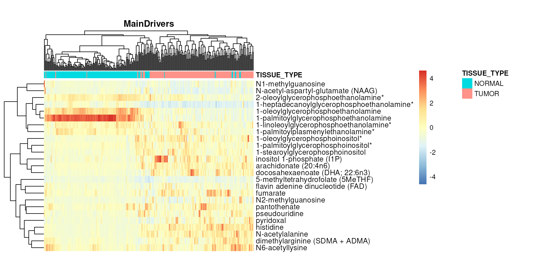

DMA

Here we use Differential Metabolite Analysis (dma) to compare two conditions (e.g. Tumour versus Healthy) by calculating the Log2FC, p-value, adjusted p-value and t-value.
For more information please see the vignette:
- Standard metabolomics data
- Consumption-Release (core) metabolomics data from cell culture media

We will perform multiple comparisons based on the different patient demographics available: 1. Tumour versus Normal: All patients 2. Tumour versus Normal: Subset of Early Stage patients 3. Tumour versus Normal: Subset of Late Stage patients 4. Tumour versus Normal: Subset of Young patients 5. Tumour versus Normal: Subset of Old patients

# Prepare the different selections
EarlyStage <- Tissue_Norm %>%
filter(STAGE== "EARLY-STAGE")
LateStage <- Tissue_Norm %>%
filter(STAGE=="LATE-STAGE")
Old <- Tissue_Norm %>%
filter(AGE=="Old")
Young <- Tissue_Norm %>%
filter(AGE=="Young")

DFs <- list(
    "TissueType" = Tissue_Norm,
    "EarlyStage" = EarlyStage,
    "LateStage" = LateStage,
    "Old" = Old,
    "Young" = Young
)

# Run dma
ResList <- list()
for(item in names(DFs)){
    #Get the right DF:
    data <- DFs[[item]]

    message(paste("Running dma for", item))
    #Create folder for saving each comparison
    dir.create(paste(getwd(),"/MetaProViz_Results/dma/", sep=""), showWarnings = FALSE)
    dir.create(paste(getwd(),"/MetaProViz_Results/dma/", item, sep=""), showWarnings = FALSE)

    #Perform dma
    TvN <- dma(data =  data[,-c(1:13)],
    metadata_sample =  data[,c(1:13)],
    metadata_info = c(Conditions="TISSUE_TYPE", Numerator="TUMOR" , Denominator = "NORMAL"),
    shapiro=FALSE, #The data have been normalized by the company that provided the results and include metabolites with zero variance as they were all imputed with the same missing value.
    path = paste(getwd(),"/MetaProViz_Results/dma/", item, sep=""))

    #Add Results to list
    ResList[[item]] <- TvN
}
#> Running dma for TissueType
#> There are no NA/0 values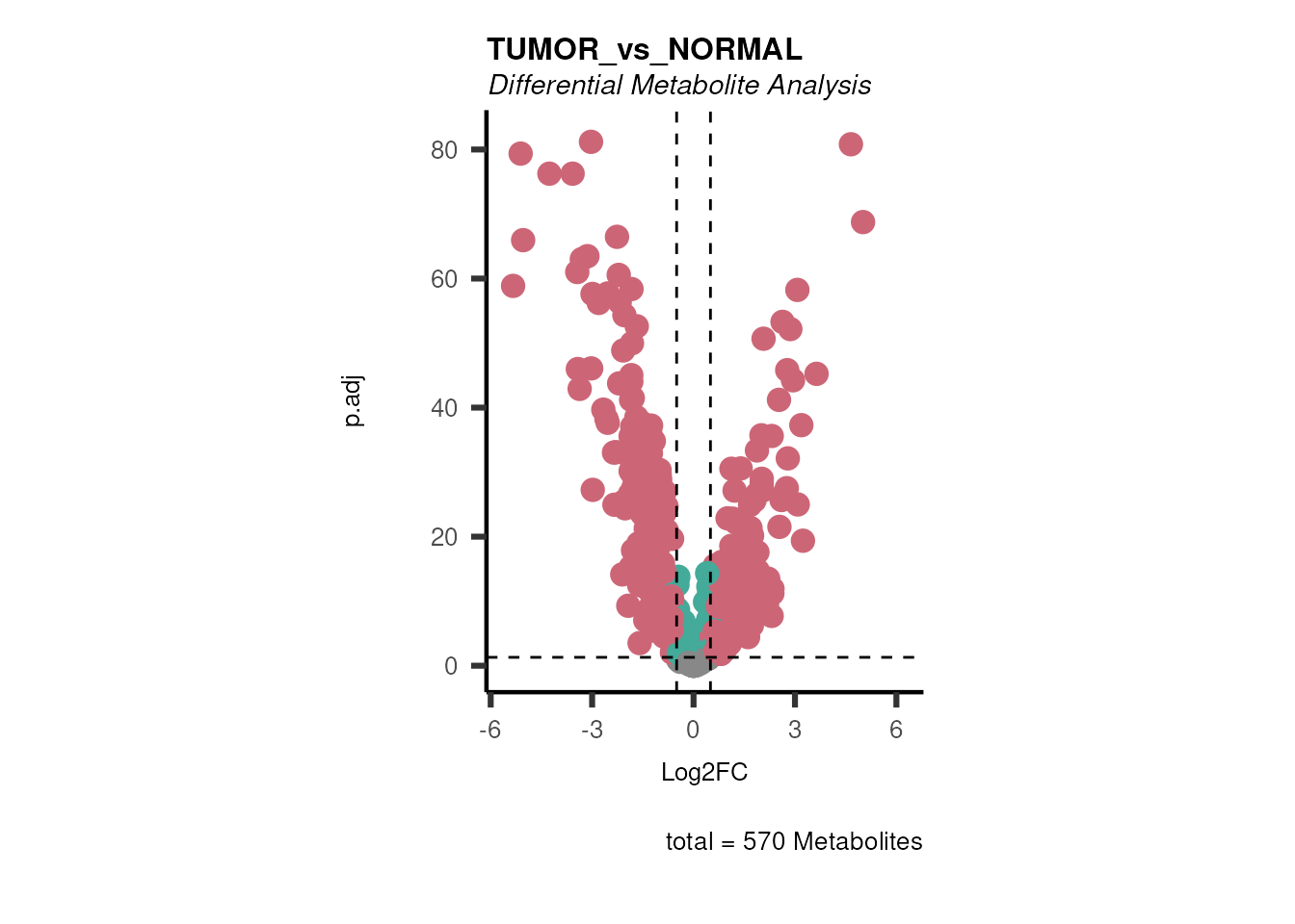

#> Running dma for EarlyStage
#> There are no NA/0 values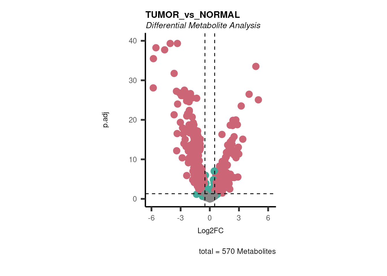

#> Running dma for LateStage
#> There are no NA/0 values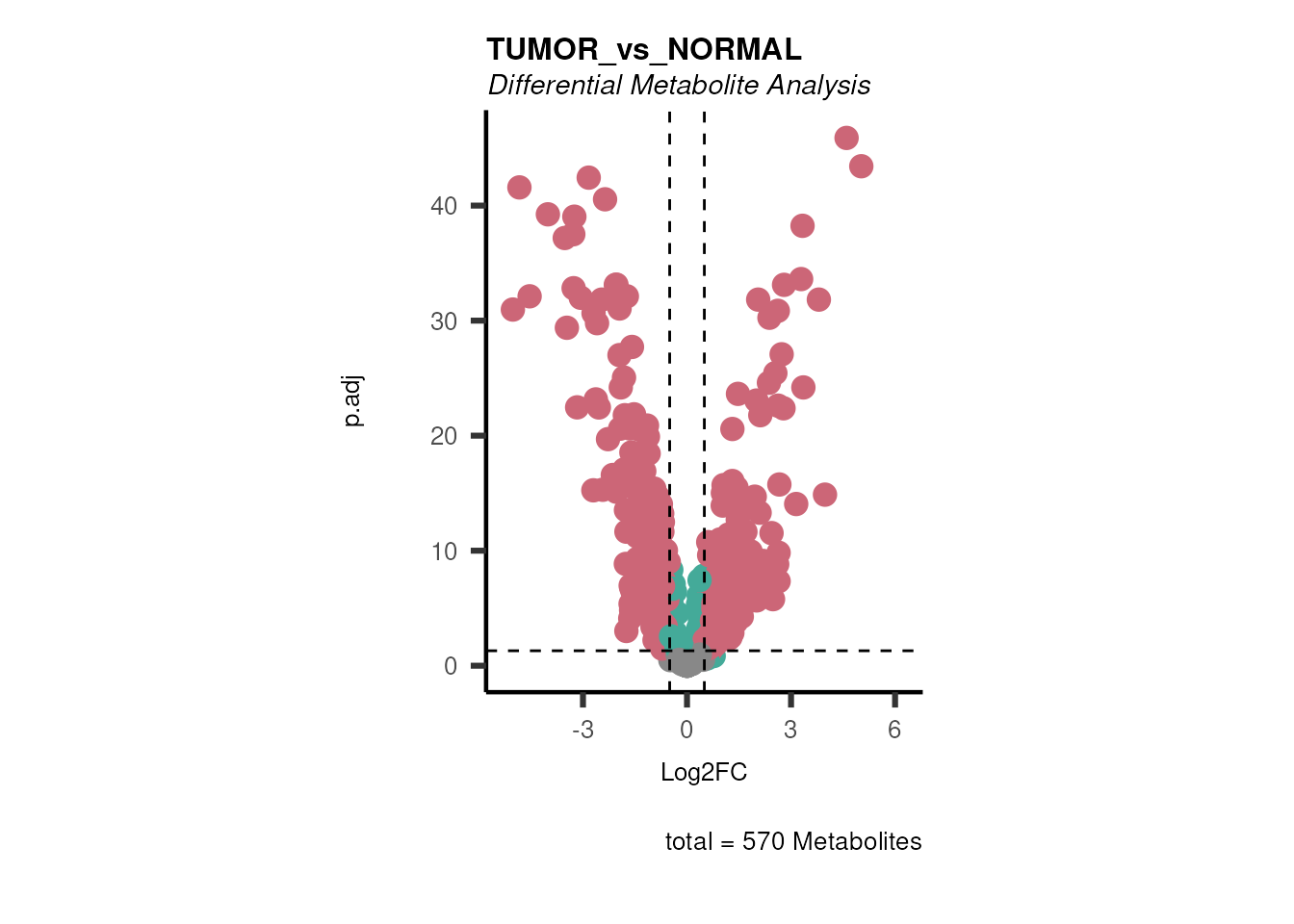

#> Running dma for Old
#> There are no NA/0 values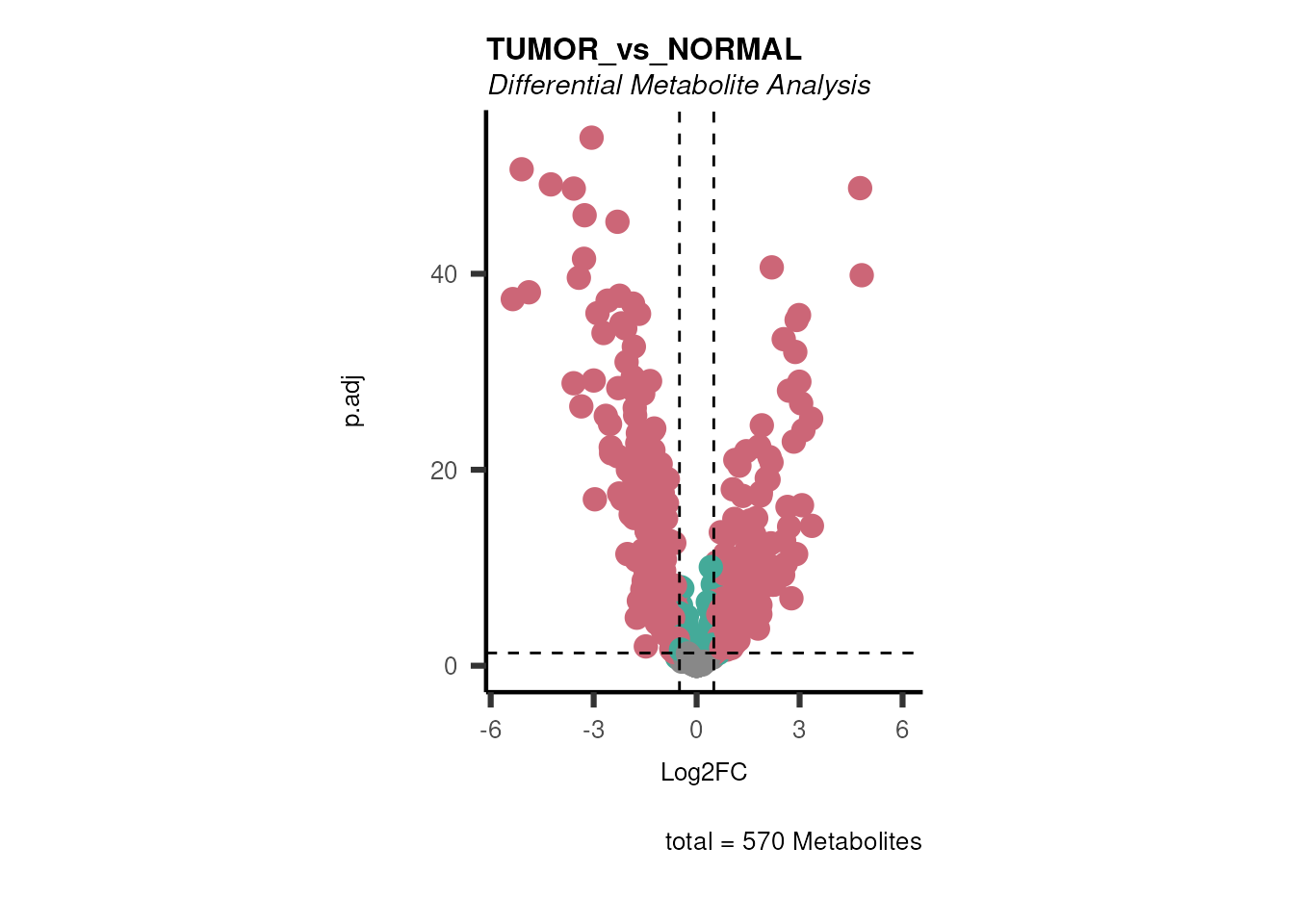

#> Running dma for Young
#> There are no NA/0 values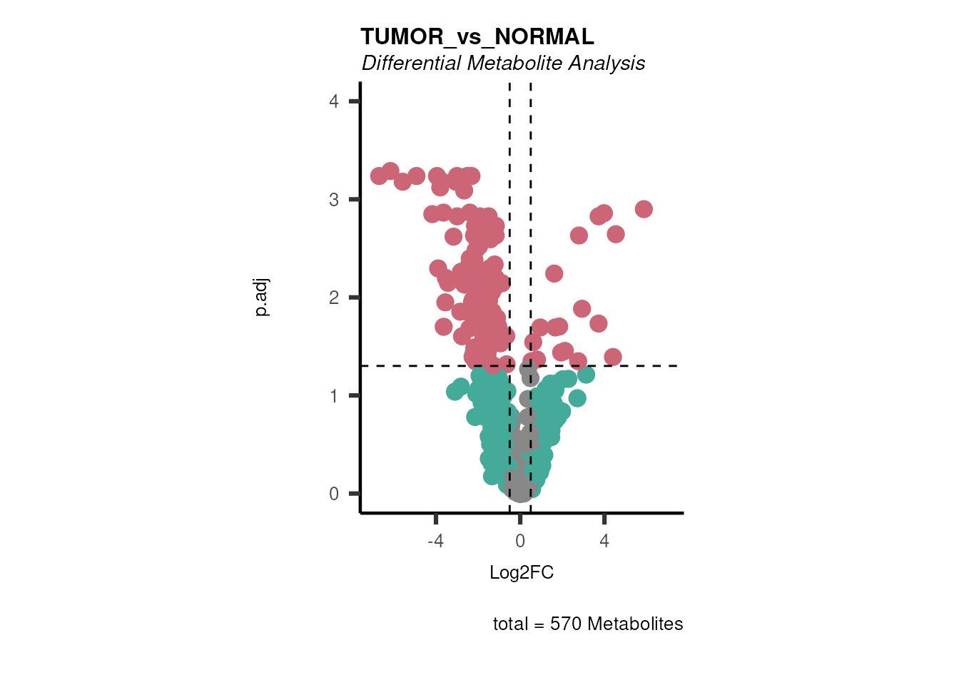

We can see from the different Volcano plots have smaller p.adjusted values and differences in Log2FC range.
Here we can also use the MetaProViz::viz_volcano() function to plot comparisons together on the same plot, such as Tumour versus Normal of young and old patients:

# Early versus Late Stage
viz_volcano(plot_types="Compare",
data=ResList[["EarlyStage"]][["dma"]][["TUMOR_vs_NORMAL"]]%>%tibble::column_to_rownames("Metabolite"),
data2= ResList[["LateStage"]][["dma"]][["TUMOR_vs_NORMAL"]]%>%tibble::column_to_rownames("Metabolite"),
name_comparison= c(data="EarlyStage", data2= "LateStage"),
plot_name= "EarlyStage-TUMOR_vs_NORMAL compared to LateStage-TUMOR_vs_NORMAL",
subtitle= "Results of dma" )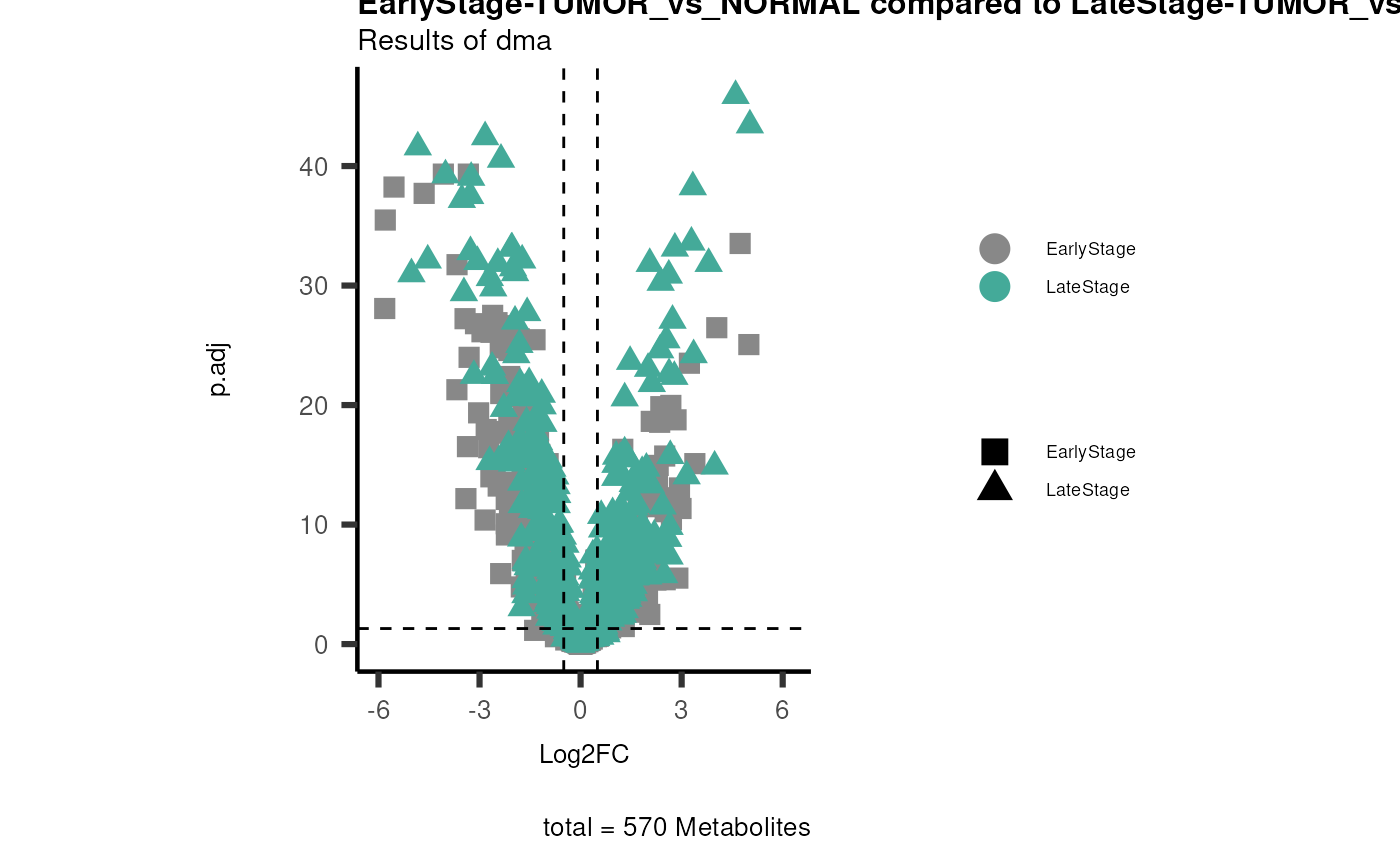


# Young versus Old
viz_volcano(plot_types="Compare",
data=ResList[["Young"]][["dma"]][["TUMOR_vs_NORMAL"]]%>%tibble::column_to_rownames("Metabolite"),
data2= ResList[["Old"]][["dma"]][["TUMOR_vs_NORMAL"]]%>%tibble::column_to_rownames("Metabolite"),
name_comparison= c(data="Young", data2= "Old"),
plot_name= "Young-TUMOR_vs_NORMAL compared to Old-TUMOR_vs_NORMAL",
subtitle= "Results of dma" )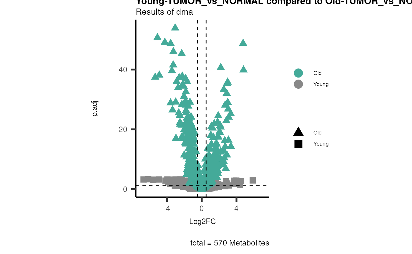

Here we can observe that Tumour versus Normal has lower significance values for the Young patients compared to the Old patients. This can be due to higher variance in the metabolite measurements from Young patients compared to the Old patients.
We can also check if the top changed metabolites comparing Tumour versus Normal correlate with the main metabolite drivers that separate patients based on their TISSUE_TYPE, which are Tumour or Normal.

# Get the top changed metabolites
top_entries <- ResList[["TissueType"]][["dma"]][["TUMOR_vs_NORMAL"]] %>%
arrange(desc(t.val)) %>%
slice(1:25)%>%
select(Metabolite)%>%
pull()
bottom_entries <- ResList[["TissueType"]][["dma"]][["TUMOR_vs_NORMAL"]] %>%
arrange(desc(t.val)) %>%
slice((n()-24):n())%>%
select(Metabolite)  %>%
pull()

# Check if those overlap with the top demographics drivers
ggVennDiagram::ggVennDiagram(list(top = top_entries,
Bottom = bottom_entries,
TissueTypeList = TissueTypeList))+
ggplot2::scale_fill_gradient(low = "blue", high = "red")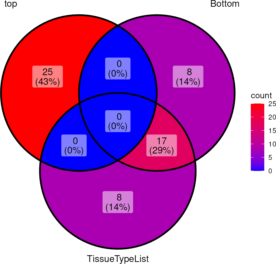

MetaData_Metab <- merge(x=tissue_meta,
y= MetaRes[["res_summary"]][, c(1,5:6) ]%>%tibble::column_to_rownames("feature"),
by=0,
all.y=TRUE)%>%
column_to_rownames("Row.names")

# Make a Volcano plot:
viz_volcano(plot_types="Standard",
data=ResList[["TissueType"]][["dma"]][["TUMOR_vs_NORMAL"]]%>%tibble::column_to_rownames("Metabolite"),
metadata_feature =  MetaData_Metab,
metadata_info = c(color = "MainDriver_Term"),
plot_name= "TISSUE_TYPE-TUMOR_vs_NORMAL",
subtitle= "Results of dma" )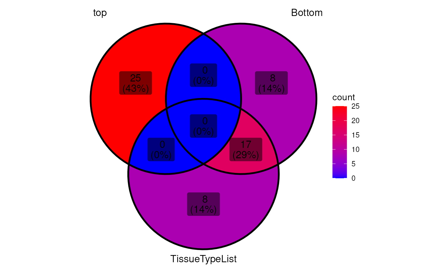

Metabolite ID QC

Before we perform enrichment analysis, it is important to check the availability of metabolite IDs that we aim to use. We can first create an overview plot:

#> Warning: `aes_string()` was deprecated in ggplot2 3.0.0.
#> ℹ Please use tidy evaluation idioms with `aes()`.
#> ℹ See also `vignette("ggplot2-in-packages")` for more information.
#> ℹ The deprecated feature was likely used in the MetaProViz package.
#>   Please report the issue at <https://github.com/saezlab/MetaProViz/issues>.
#> This warning is displayed once per session.
#> Call `lifecycle::last_lifecycle_warnings()` to see where this warning was
#> generated.

Here we notice that 76 features have no metabolite ID assigned, yet have a trivial name and a metabolite class assigned. For 135 metabolites we only have a pubchem ID, yet no HMDB or KEGG ID. Next, we will try to understand the missing IDs focusing on HMDB as an example:

Plot1_HMDB <- count_id(MetaboliteIDs, "HMDB",  delimiter = ";")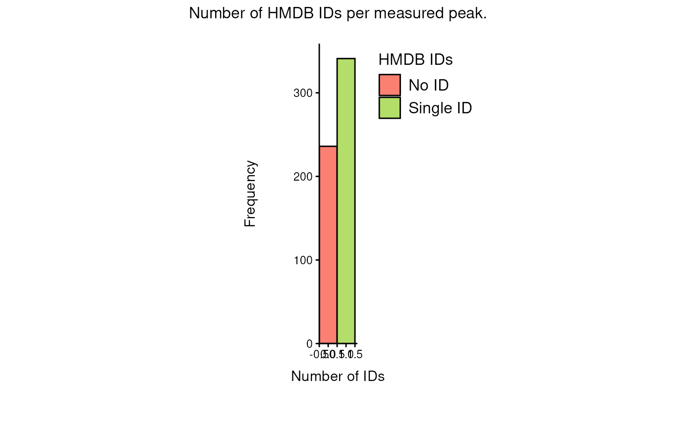

Over 200 metabolites have no HMDB ID and if there is a HMDB ID assigned, we only have one HMDB ID. Here we assume the experimental setup does not account for stereoisomers and that other IDs are with different degrees of ambiguity are possible (e.g. L-Alanine HMDB ID is present and we will add D-Alanine HMDB ID later, see PK vignette for more details). This enables us to assign additional potential HMDB IDs per feature.

Additionally, for the metabolites without HMDB ID we can check if a HMDB ID is available using the other ID types. First we check if we have cases in which we do have no HMDB ID, but other available IDs:

Overview of other ID types for metabolites without HMDB ID.
Total_Cases	Not_NA_PUBCHEM	Not_NA_KEGG	Both_Not_NA
160	159	25	24

To unravel such issues in a structured way and solve them at the same time, MetaProViz offers a complete id_processing() workflow function, performing multiple steps at once: Initial quality control and ID assessment - Count present ID types in an Upset plot, like we just saw - Assess how many IDs are present per feature, for multiple ID types at once, such as HMDB, KEGG, ChEBI and PubChem. - perform compatibility check of present IDs, i.e. asking whether all present IDs per feature correspond to the same metabolite or whether there are errors in the present annotations. Automatically filters out incompatible metabolite IDs per feature Subsequent controlled expansion of the ID space - using ID traversal (using a graph-based translation approach) to increase ID coverage per feature - performing quantification per step of the workflow

For a more detailed tutorial of the id_processing() function, visit the id-processing-workflow vignette


MetaboliteIDs_processed <- 
    id_processing(
        MetaboliteIDs,
        id_types = c("HMDB", "KEGG", "CHEBI", "PUBCHEM"),
        delimiter = ";",
        run_compatibility_check = TRUE,
        handle_partially_compatible = TRUE,
        handle_completely_incompatible = TRUE,
        completely_incompatible_priority = c("KEGG", "HMDB", "CHEBI", "PUBCHEM"), # in case of incompatible IDs, retain KEGG so we can better perform KEGG ORA later
        run_traversal = TRUE,
        compare_name_col = "Metabolite",
        print_plot = FALSE
    )
#> [id_processing] Starting workflow on 577 feature(s).
#> [id_processing] Selected namespaces: HMDB, KEGG, CHEBI, PUBCHEM
#> [id_processing] Steps enabled: compatibility=TRUE, translation=FALSE, traversal=TRUE
#> [id_processing] Defaults/assumptions: partial_auto=TRUE, complete_auto=TRUE, complete_priority=KEGG > HMDB > CHEBI > PUBCHEM
#> [id_processing] Quantifying ID space for stage 'input'.
#> [id_processing] Running seed_id_compatibility_check().
#> seed_id_compatibility_check() ID-handling choices:
#> - handle_partially_compatible: TRUE
#> - handle_completely_incompatible: TRUE
#> seed_id_compatibility_check() returned:
#> - ID_pair_compatibility: raw seed-ID pair QC table.
#> - data_with_compatibility: input feature table with raw compatibility flag.
#> - feature_compatibility_summary: one row per feature with QC class and counts.
#> - data_after_handling: cleaned feature table after optional automatic handling.
#> - ID_pair_compatibility_after_handling: pair QC recomputed from cleaned IDs.
#> - handling_summary_text / handling_summary_metrics: concise summary of handling choices and effects.
#> [id_processing] Quantifying ID space for stage 'after_compatibility'.
#> [id_processing] Running traverse_ids().
#> Warning: Unknown or uninitialised column: `all_seed_ids_compatible`.
#> [id_processing] Quantifying ID space for stage 'after_traversal'.
#> [id_processing] Stage 'input': HMDB total_ids=343 no_id=236 single=339 multiple=2 | KEGG total_ids=312 no_id=271 single=301 multiple=5 | CHEBI total_ids=0 no_id=577 single=0 multiple=0 | PUBCHEM total_ids=503 no_id=120 single=420 multiple=37
#> [id_processing] Stage 'after_compatibility': HMDB total_ids=322 no_id=255 single=322 multiple=0 | KEGG total_ids=299 no_id=284 single=288 multiple=5 | CHEBI total_ids=0 no_id=577 single=0 multiple=0 | PUBCHEM total_ids=458 no_id=155 single=395 multiple=27
#> [id_processing] Stage 'after_traversal': HMDB total_ids=727 no_id=120 single=298 multiple=159 | KEGG total_ids=325 no_id=263 single=304 multiple=10 | CHEBI total_ids=752 no_id=160 single=188 multiple=229 | PUBCHEM total_ids=713 no_id=96 single=348 multiple=133
#> [id_processing] Workflow steps run: initial_exploration -> compatibility_check -> traversal. Returned Data tables: input, after_compatibility, after_traversal. Returned Plot stages: input, after_compatibility, after_traversal. Final stage 'after_traversal' contains 577 feature(s).
#> [id_processing] Suggestion: equivalent_id() is not part of this workflow yet. If you want additional ambiguity-aware within-namespace expansion, run it afterwards on the final feature metadata.

After running the automatic id_processing, we can additionally add stereochemically equivalent IDs to the already expanded feature space. Due to the missing complete resolution in most mass spectrometry based metabolite acquisition methods, we may have L- or D- amino acid or R-/S- sugar IDs present for some features. However, if we cannot be sure of which version we annotated, we must add the respective counterparts to match features to prior knowledge in a stable way.

#> chebi is used to find additional potential IDs for hmdb.
#> chebi is used to find additional potential IDs for kegg.
#> pubchem is used to find additional potential IDs for chebi.
#> chebi is used to find additional potential IDs for pubchem.
#>         before after added
#> HMDB       727   744    17
#> KEGG       325   325     0
#> CHEBI      752   816    64
#> PUBCHEM    713   759    46

Lastly, we will have the new metadata table, which we can use for enrichment analysis:

If we compare the results to the upset plot from the original metadata we can see that initially 251 metabolites had a pubchem, HMDB and KEGG ID, whilst we now see 292 features covered by HMDB, PUBCHEM, CHEBI and KEGG IDs at the same time, a notable increase in coverage. Additional 115 features carry PUBCHEM, HMDB and CHEBI IDs. 135 metabolite had only a Pubchem ID, whilst now only 26 metabolites remaining with only a Pubchem ID. With this increase in ID coverage for many features, we now have better possibilities to map our experimental data to diverse sets of Prior Knowledge to perform downstream analyses.

ORA

We can perform Over Representation Analysis (ORA) using KEGG pathways for each comparison and plot significant pathways. Noteworthy, since not all metabolites have KEGG IDs, we will lose information.

Given that in some cases we have multiple KEGG IDs for a measured feature, we will check if this causes mapping to multiple, different entries in the KEGG pathway-metabolite sets:

#Load Kegg pathways:
KEGG_Pathways <- metsigdb_kegg()

Tissue_MetaData_Extended <- Tissue_MetaData_Extended |>
  dplyr::mutate(dplyr::across(c(HMDB, KEGG, CHEBI, PUBCHEM), ~ gsub("\\s*;\\s*", ", ", .x)))

#check mapping with metadata
ccRCC_to_KEGGPathways <- checkmatch_pk_to_data(data = Tissue_MetaData_Extended,
                                               input_pk = KEGG_Pathways,
                                               metadata_info = c(InputID = "KEGG", PriorID = "MetaboliteID", grouping_variable = "term"))
#> Warning in checkmatch_pk_to_data(data = Tissue_MetaData_Extended, input_pk =
#> KEGG_Pathways, : 263 NA values were removed from column KEGG
#> Warning in checkmatch_pk_to_data(data = Tissue_MetaData_Extended, input_pk =
#> KEGG_Pathways, : 5 duplicated IDs were removed from column KEGG
#> data has multiple IDs per measurement = TRUE. input_pk has multiple IDs per entry = FALSE.
#> data has 309 unique entries with 320 unique KEGG IDs. Of those IDs, 249 match, which is 77.8125%.
#> input_pk has 6645 unique entries with 6645 unique MetaboliteID IDs. Of those IDs, 249 are detected in the data, which is 3.74717832957111%.
#> Warning in checkmatch_pk_to_data(data = Tissue_MetaData_Extended, input_pk =
#> KEGG_Pathways, : There are cases where multiple detected IDs match to multiple
#> prior knowledge IDs of the same category

problems_terms <- ccRCC_to_KEGGPathways[["GroupingVariable_summary"]]%>%
    filter(!Group_Conflict_Notes== "None")

Terms in KEGG pathways where the same measured feature maps with more than one ID, which will inflate the enrichment analysis.
KEGG	original_count	matches_count	InputID_select	MetaboliteID
C00221, C00031	2	2	NA	C00031
C00221, C00031	2	2	NA	C00221
C00221, C00031	2	2	NA	C00221
C00221, C00031	2	2	NA	C00221
C00221, C00031	2	2	NA	C00221
C00221, C00031	2	2	NA	C00031
C00221, C00031	2	2	NA	C00031
C00221, C00031	2	2	NA	C00031
C00258, C01921	2	2	NA	C00258
C00258, C01921	2	2	NA	C01921
C03460, C03722	2	2	NA	C03460
C03460, C03722	2	2	NA	C03722
C17737, C00695	2	2	NA	C00695
C17737, C00695	2	2	NA	C17737

Dependent on the biological question and the organism and prior knowledge, one can either maintain the metabolite ID of the more likely metabolite (e.g. in human it is more likely that we have L-aminoacid than D-aminoacid) or the metabolite ID that is represented in more/less pathways (specificity). If we are looking into the cases where we do have multiple IDs, for cases with no match to the prior knowledge we can just maintain one ID, whilst for cases with exactly one match we should maintain the ID that is found in the prior knowledge.

# Select the cases where a feature has multiple IDs
multipleIDs <- ccRCC_to_KEGGPathways[["data_summary"]]%>%
filter(original_count>1)

Terms in KEGG pathways where the same measured feature maps with more than one ID, which may inflate the enrichment analysis.
KEGG	InputID_select	original_count	matches_count	matches	Group_Conflict_Notes	ActionRequired	Action_Specific
C00065, C00716	NA	2	2	C00065, C00716	None	Check	KeepEachID
C00155, C05330	C00155	2	1	C00155	None	None	None
C00221, C00031	NA	2	2	C00221, C00031	None \|\| Glycolysis / Gluconeogenesis \|\| Pentose phosphate pathway \|\| Metabolic pathways \|\| Biosynthesis of secondary metabolites	Check	KeepOneID
C00258, C01921	NA	2	2	C00258, C01921	None \|\| Metabolic pathways	Check	KeepOneID
C00671, C06008	C00671	2	1	C00671	None	None	None
C01835, C00721, C00420	NA	3	2	C01835, C00721	None	Check	KeepEachID
C01991, C00989	C00989	2	1	C00989	None	None	None
C02052, C00464	C00464	2	1	C00464	None	None	None
C03460, C03722	NA	2	2	C03460, C03722	Metabolic pathways \|\| None	Check	KeepOneID
C17737, C00695	NA	2	2	C17737, C00695	None \|\| Secondary bile acid biosynthesis	Check	KeepOneID

In case of ActionRequired=="Check", we can look into the column Action_Specific which contains additional information. In case of the entry KeepEachID, multiple matches to the prior knowledge were found, yet the features are in different pathways (=GroupingVariable). Yet, in case of KeepOneID, the different IDs map to the same pathway in the prior knowledge for at least one case and therefore keeping both would inflate the enrichment analysis.

SelectedIDs <- ccRCC_to_KEGGPathways[["data_summary"]]%>%
#Expand rows where Action == KeepEachID by splitting `matches`
dplyr::mutate(matches_split = if_else(Action_Specific == "KeepEachID", matches, NA_character_)) %>%
separate_rows(matches_split, sep = ",\\s*") %>%
mutate(InputID_select = if_else(Action_Specific  == "KeepEachID", matches_split, InputID_select)) %>%
select(-matches_split) %>%
#Select one ID for Action_Specific==KeepOneID
dplyr::mutate(InputID_select = case_when(
    Action_Specific == "KeepOneID" & matches ==  "C00221, C00031" ~ "C00031", # These are D- and L-Glucose. We have human samples, so in this conflict we will maintain L-Glucose
    Action_Specific == "KeepOneID" & matches ==  "C00258, C01921" ~ "C01921", # D-Glycerate versus Glycocholate. Other IDs also suggest Glycocholate, hence keep it.
    Action_Specific == "KeepOneID" & matches == "C03460, C03722" ~ "C03722", # 2-Methylprop-2-enoyl-CoA versus Quinolinate. No evidence, hence we keep the one present in more pathways ( C03722=7 pathways, C03460=2 pathway)
    Action_Specific == "KeepOneID" & matches ==  "C17737, C00695" ~ "C00695", # Allocholic acid versus Cholic acid. No evidence, hence we keep the one present in more pathways (C00695 = 4 pathways, C17737 = 1 pathway)
    Action_Specific == "KeepOneID" ~ InputID_select,  # Keep NA where not matched manually
    TRUE ~ InputID_select
    ))

Lastly, we need to add the column including our selected IDs to the metadata table:

Tissue_MetaData_Extended <- merge(x= SelectedIDs %>%
                                        dplyr::select(KEGG, InputID_select),
                                        y= Tissue_MetaData_Extended,
                                        by= "KEGG",
                                        all.y=TRUE)

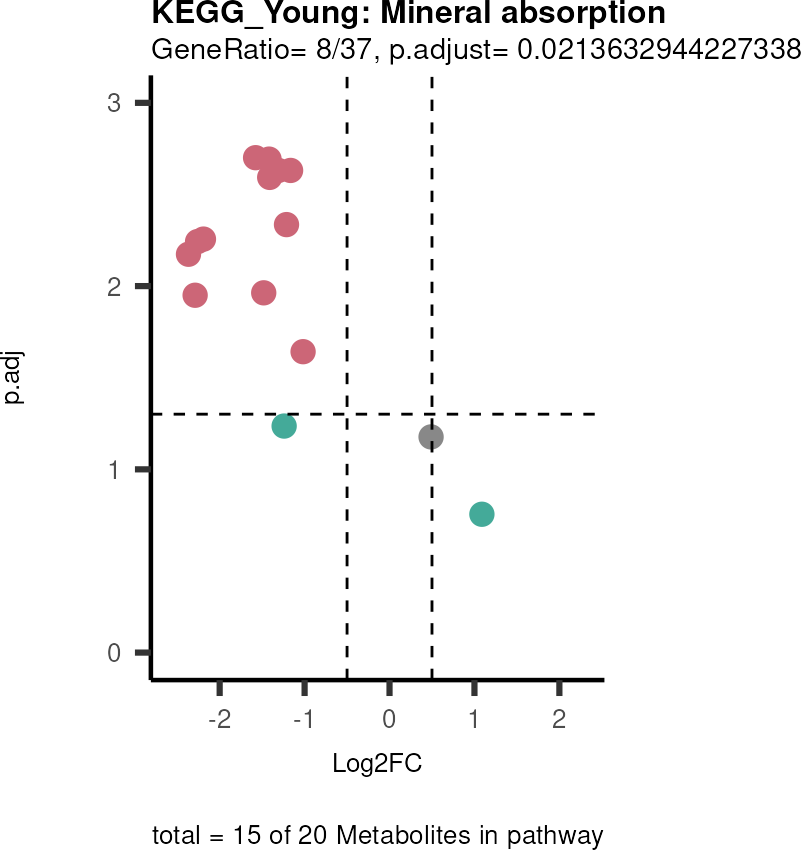
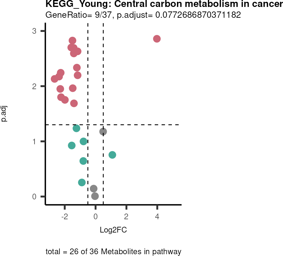
For results with p.adjusted value < 0.1 and a minimum of 10% of the pathway detected will be visualized as Volcano plots:

# Since we have performed multiple comparisons (one per patient subset), we will run ORA for each of them
DM_ORA_res<- list()

for(comparison in names(ResList)){#Res list includes the different comparisons we performed above <-
#Ensure that the Metabolite names match with KEGG IDs or KEGG trivial names.
dma_res <- merge(x= Tissue_MetaData_Extended,
y= ResList[[comparison]][["dma"]][["TUMOR_vs_NORMAL"]],
by="Metabolite",
all=TRUE)

#Ensure unique IDs and full background --> we include measured features that do not have a KEGG ID.
dma_res <- dma_res %>%
    dplyr::select(InputID_select, Log2FC, p.val, p.adj, t.val) %>%
    dplyr::mutate(InputID_select = if_else(
        is.na(InputID_select),
        paste0("NA_", cumsum(is.na(InputID_select))),
        InputID_select
        ))%>% #remove duplications and keep the higher Log2FC measurement
    group_by(InputID_select) %>%
    slice_max(order_by = Log2FC, n = 1, with_ties = FALSE) %>%
    ungroup()%>%
    remove_rownames()%>%
    tibble::column_to_rownames("InputID_select")

    #Perform ORA
    Res <- standard_ora(data= dma_res, #Input data requirements: column `t.val` and column `Metabolite`
    metadata_info=c(pvalColumn="p.adj", percentageColumn="t.val", PathwayTerm= "term", PathwayFeature= "MetaboliteID"),
    input_pathway=KEGG_Pathways,#Pathway file requirements: column `term`, `Metabolite` and `Description`. Above we loaded the KEGG_Pathways using metsigdb_kegg()
    pathway_name=paste0("KEGG_", comparison, sep=""),
    min_gssize=3,
    max_gssize=1000,
    cutoff_stat=0.01,
    cutoff_percentage=10)

    DM_ORA_res[[comparison]] <- Res

    #Select to plot:
    Res_Select <- Res[["ClusterGosummary"]]%>%
    filter(p.adjust<0.1)%>%
    #filter(pvalue<0.05)%>%
    filter(percentage_of_Pathway_detected>10)

    if(is.null(Res_Select)==FALSE){
        viz_volcano(plot_types="PEA",
        data= dma_res, #Must be the data you have used as an input for the pathway analysis
        data2=as.data.frame(Res_Select )%>%dplyr::rename("term"="ID"),
        metadata_info= c(PEA_Pathway="term",# Needs to be the same in both, metadata_feature and data2.
        PEA_stat="p.adjust",#Column data2
        PEA_score="GeneRatio",#Column data2
        PEA_Feature="MetaboliteID"),# Column metadata_feature (needs to be the same as row names in data)
        metadata_feature= KEGG_Pathways,#Must be the pathways used for pathway analysis
        plot_name= paste("KEGG_", comparison, sep=""),
        subtitle= "PEA" )
        }
}

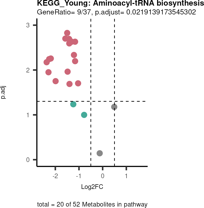
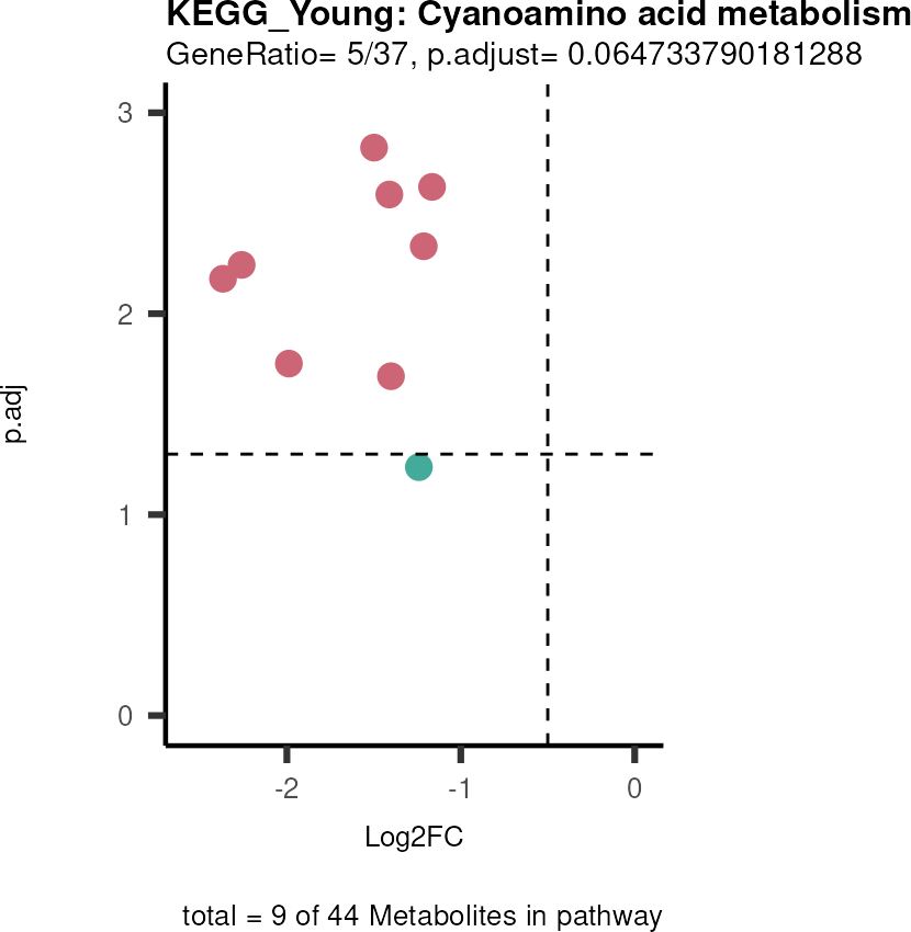
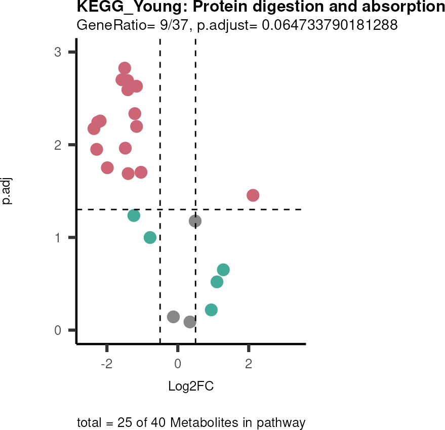
Biological regulated clustering

To understand which metabolites are changing independent of the patients age, hence only due to tumour versus normal, and which metabolites change independent of tumour versus normal, hence due to the different age, we can use the mca_2cond() function.
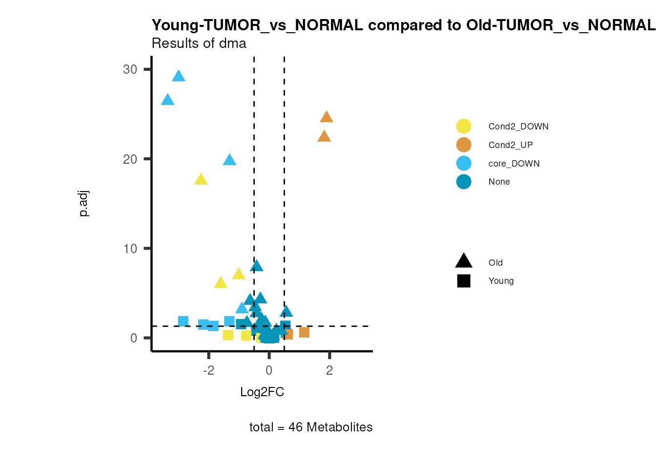
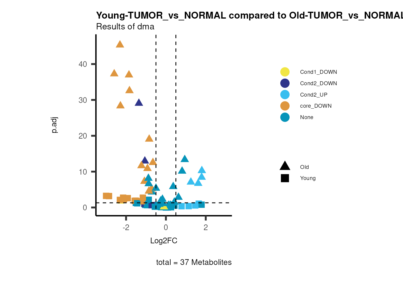
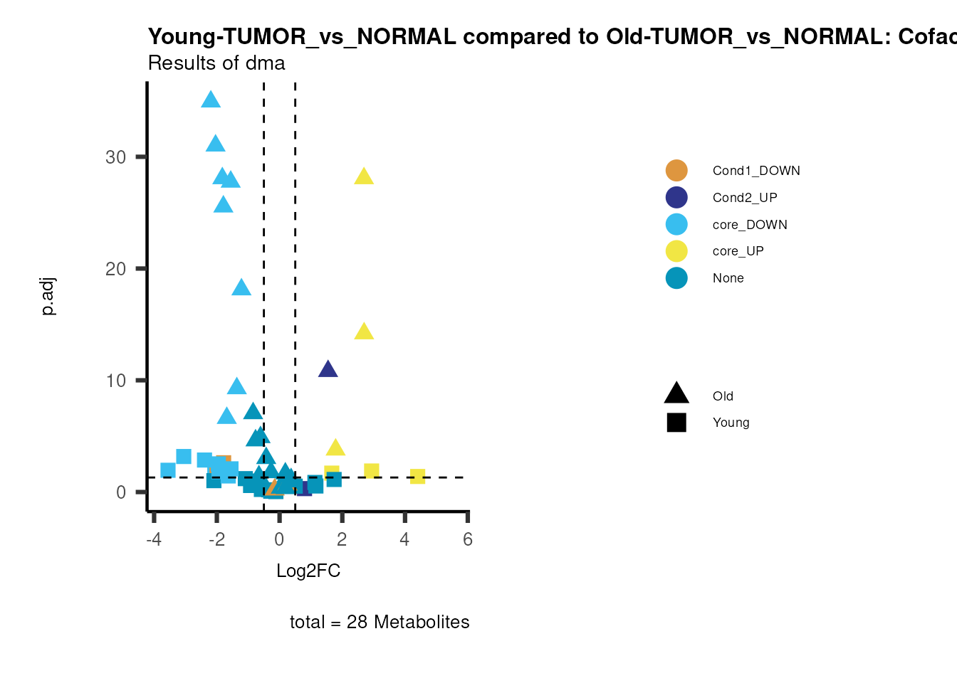
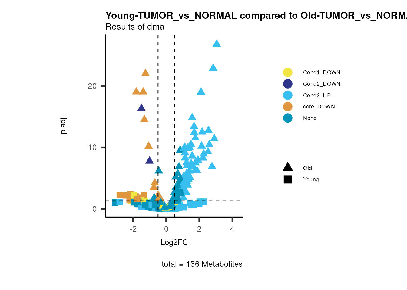
Metabolite Clustering Analysis (MCA) enables clustering of metabolites into groups based on logical regulatory rules. Here we set two different thresholds, one for the differential metabolite abundance (Log2FC) and one for the significance (e.g. p.adj). This will define if a feature (= metabolite) is assigned into:
1. “UP”, which means a metabolite is significantly up-regulated in the underlying comparison.
2. “DOWN”, which means a metabolite is significantly down-regulated in the underlying comparison.
3. “No Change”, which means a metabolite does not change significantly in the underlying comparison and/or is not defined as up-regulated/down-regulated based on the Log2FC threshold chosen.

Thereby “No Change” is further subdivided into four states:
1. “Not Detected”, which means a metabolite is not detected in the underlying comparison.
2. “Not Significant”, which means a metabolite is not significant in the underlying comparison.
3. “Significant positive”, which means a metabolite is significant in the underlying comparison and the differential metabolite abundance is positive, yet does not meet the threshold set for “UP” (e.g. Log2FC >1 = “UP” and we have a significant Log2FC=0.8).
4. “Significant negative”, which means a metabolite is significant in the underlying comparison and the differential metabolite abundance is negative, yet does not meet the threshold set for “DOWN”.

For more information you can also check out the other vignettes.

MCAres <-  mca_2cond(data_c1=ResList[["Young"]][["dma"]][["TUMOR_vs_NORMAL"]],
data_c2=ResList[["Old"]][["dma"]][["TUMOR_vs_NORMAL"]],
metadata_info_c1=c(ValueCol="Log2FC",StatCol="p.adj", cutoff_stat= 0.05, ValueCutoff=1),
metadata_info_c2=c(ValueCol="Log2FC",StatCol="p.adj", cutoff_stat= 0.05, ValueCutoff=1),
feature = "Metabolite",
save_table = "csv",
method_background="C1&C2"#Most stringent background setting, only includes metabolites detected in both comparisons
)

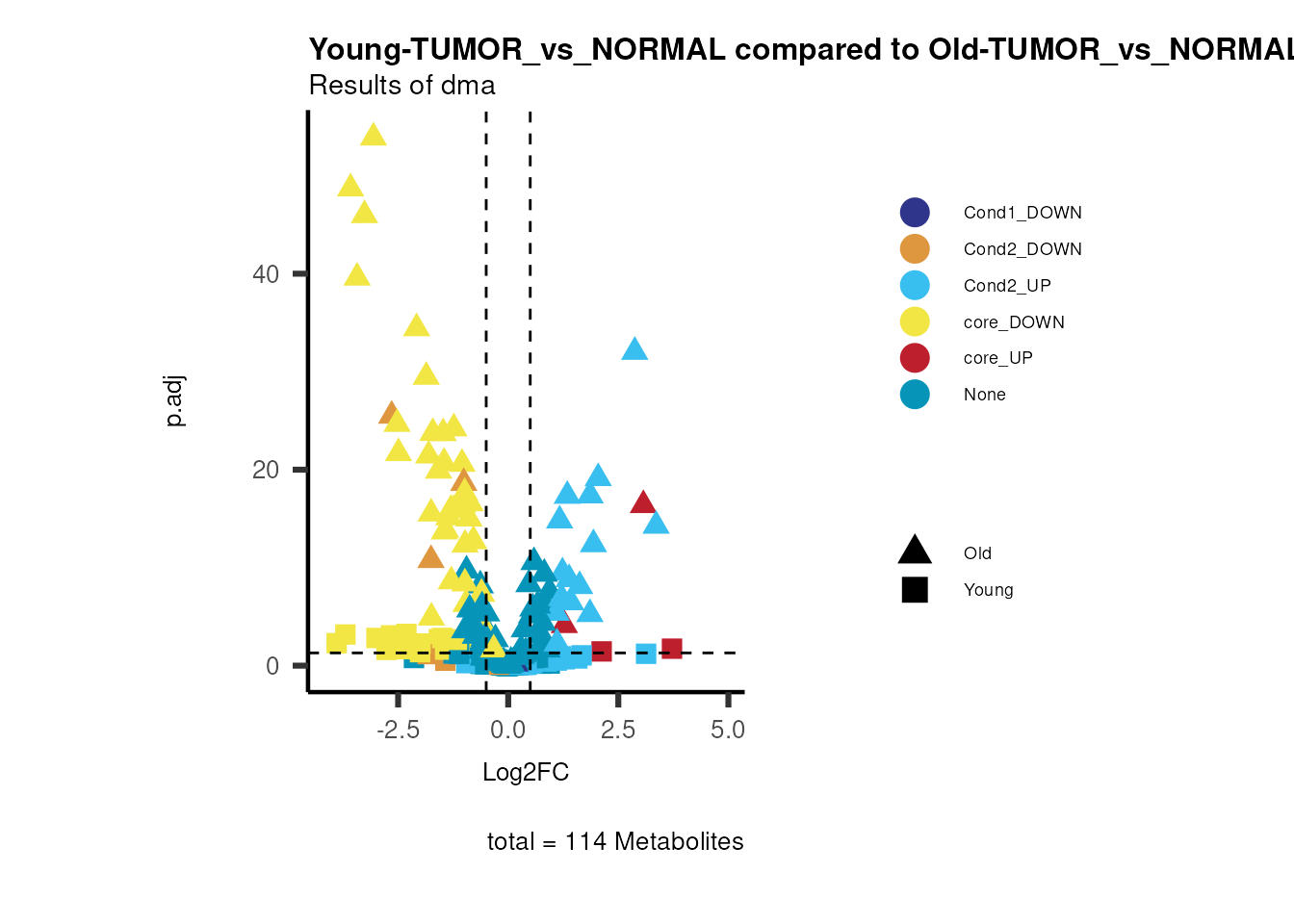
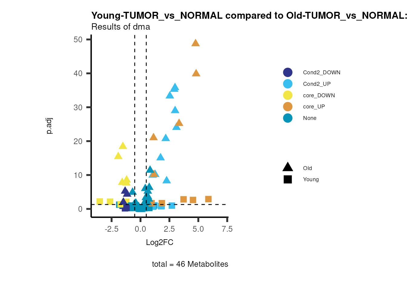
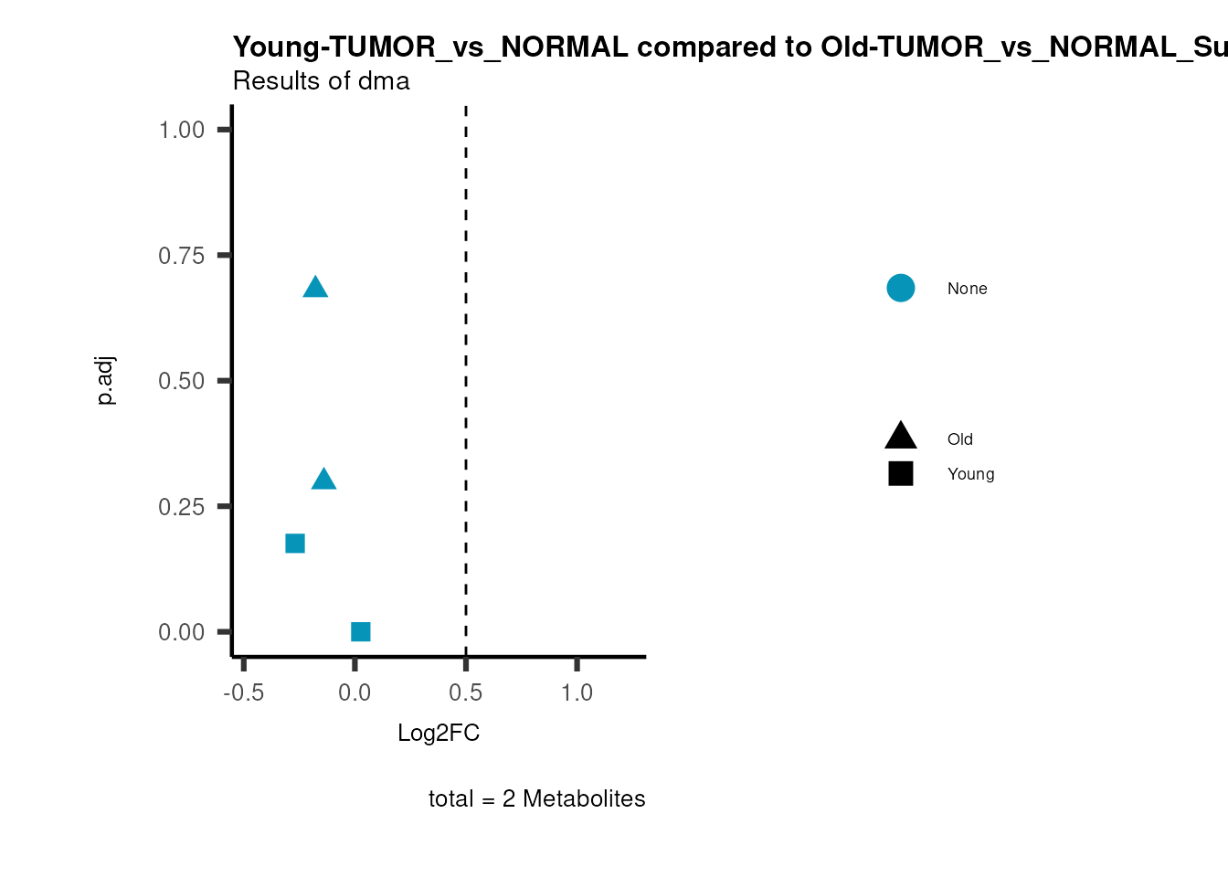
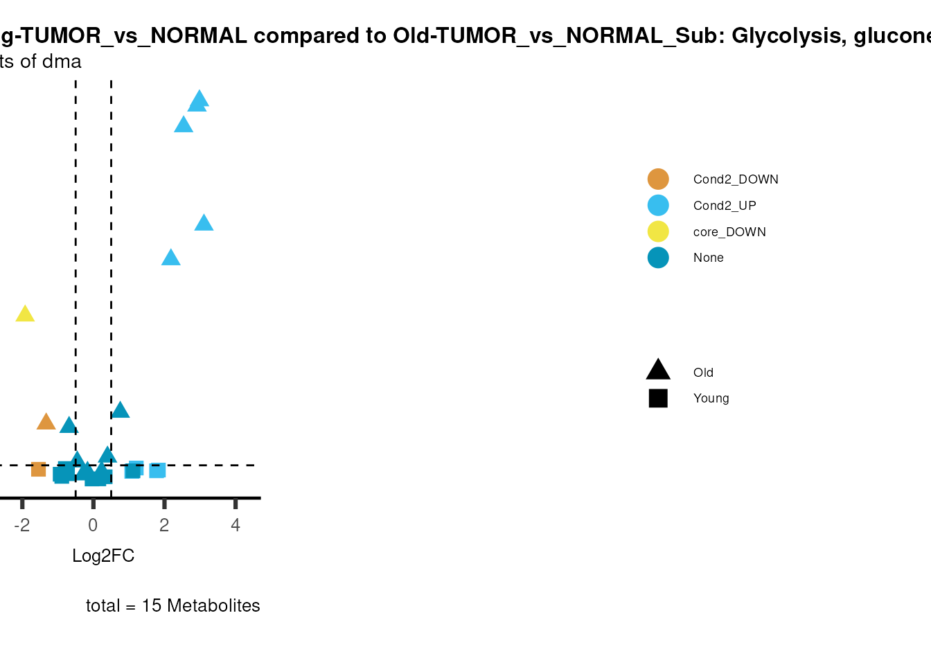
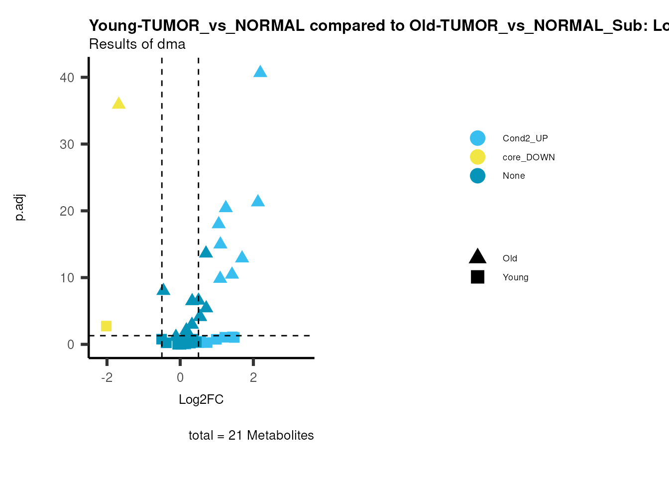
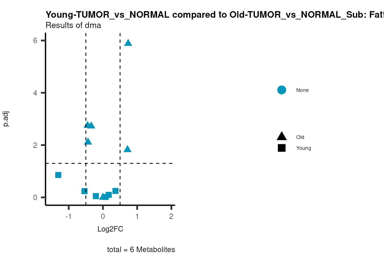
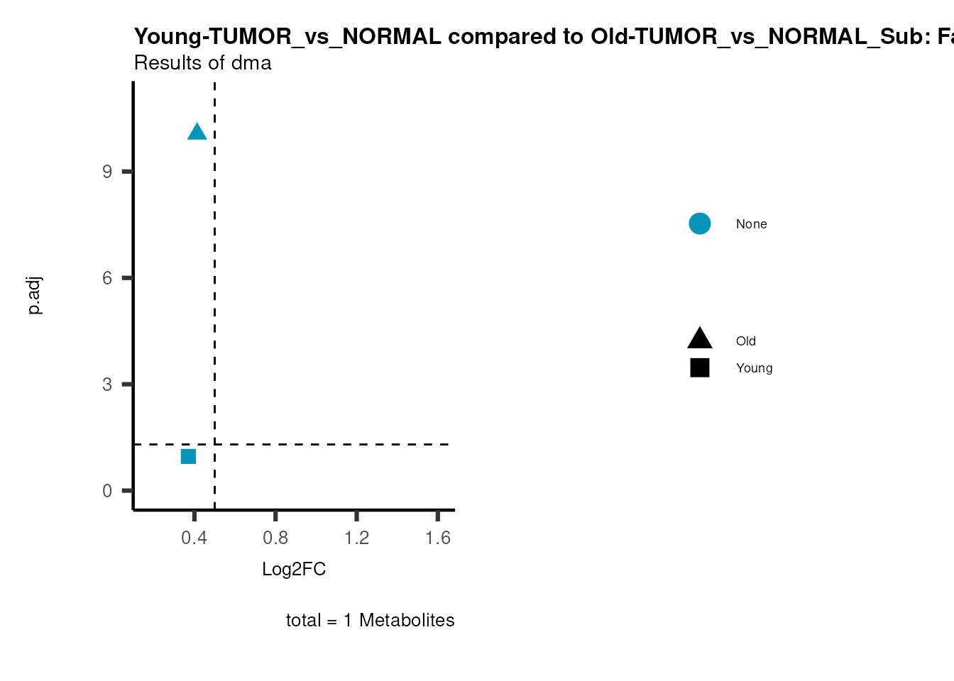
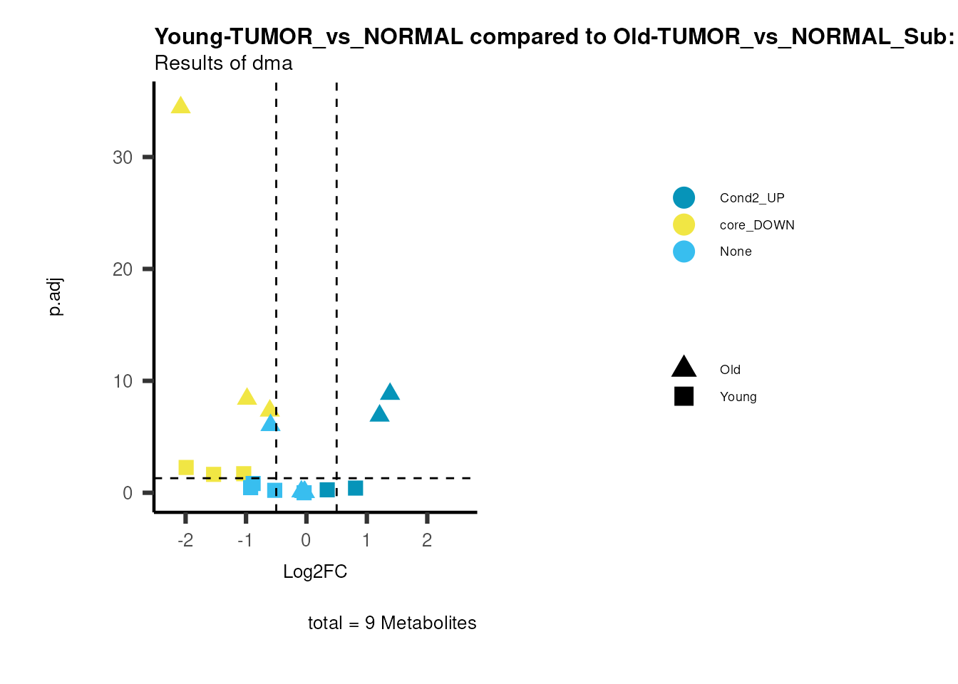
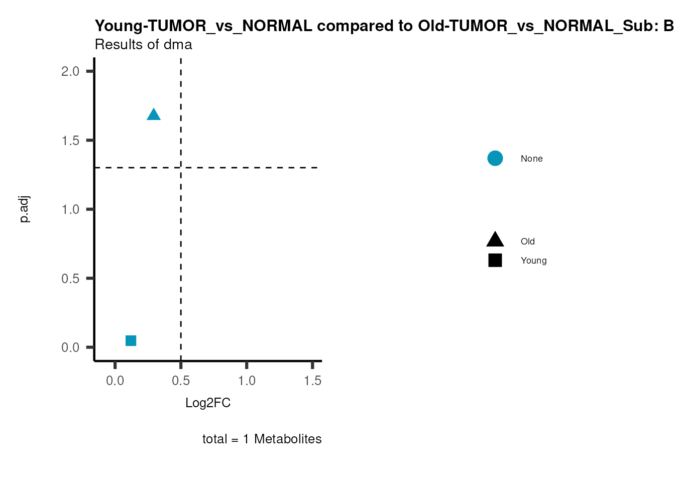
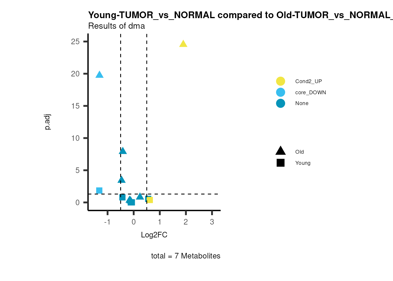
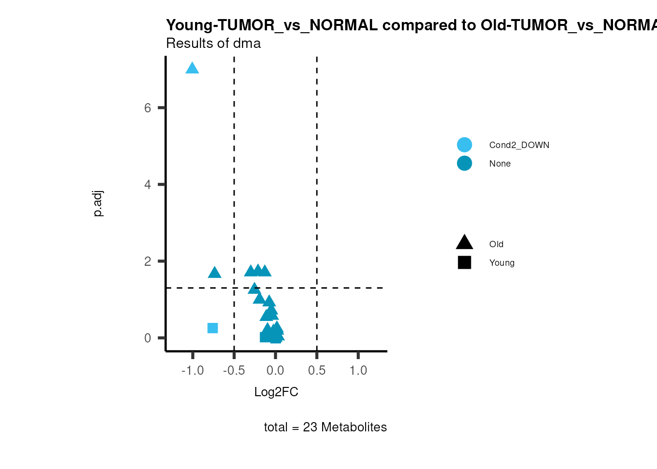
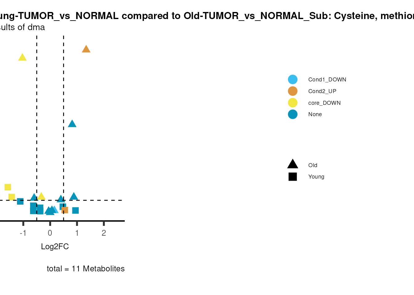
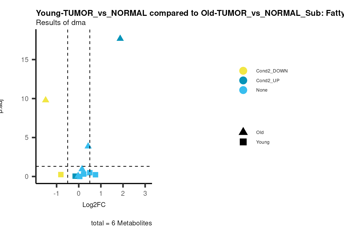
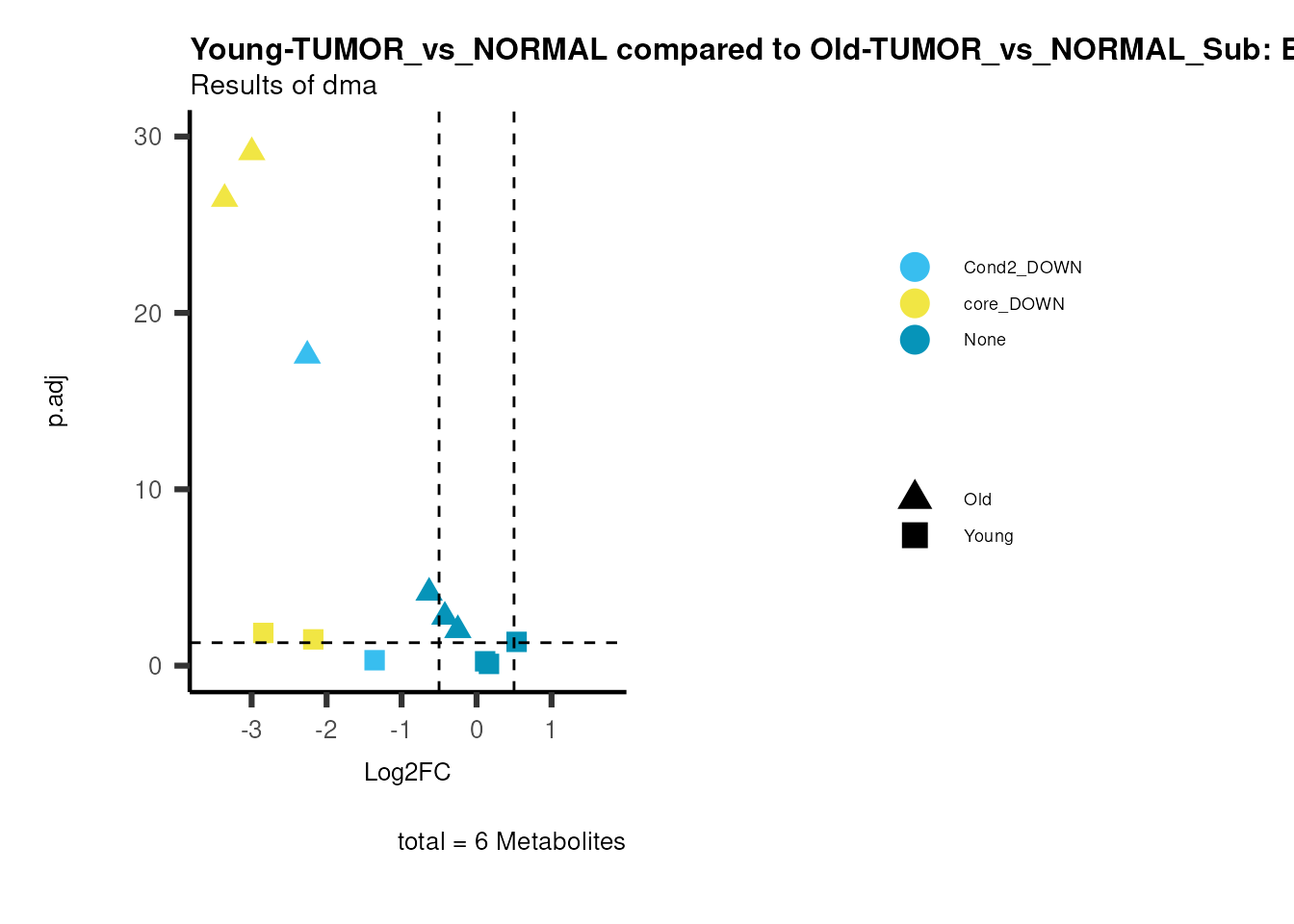
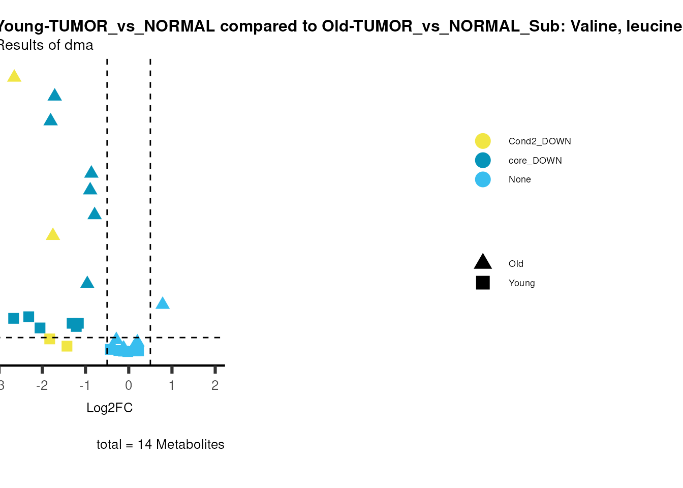
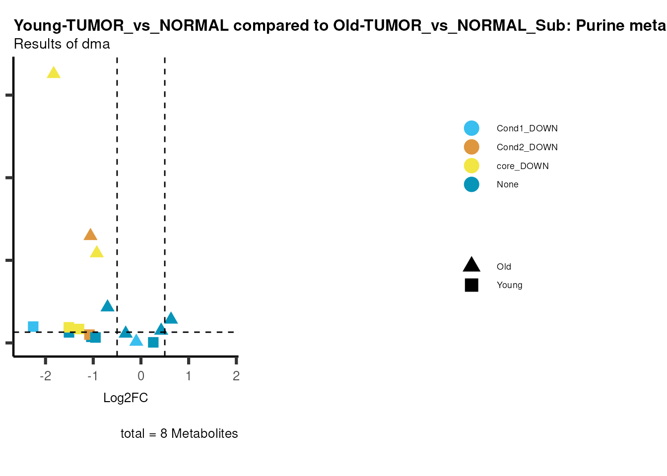
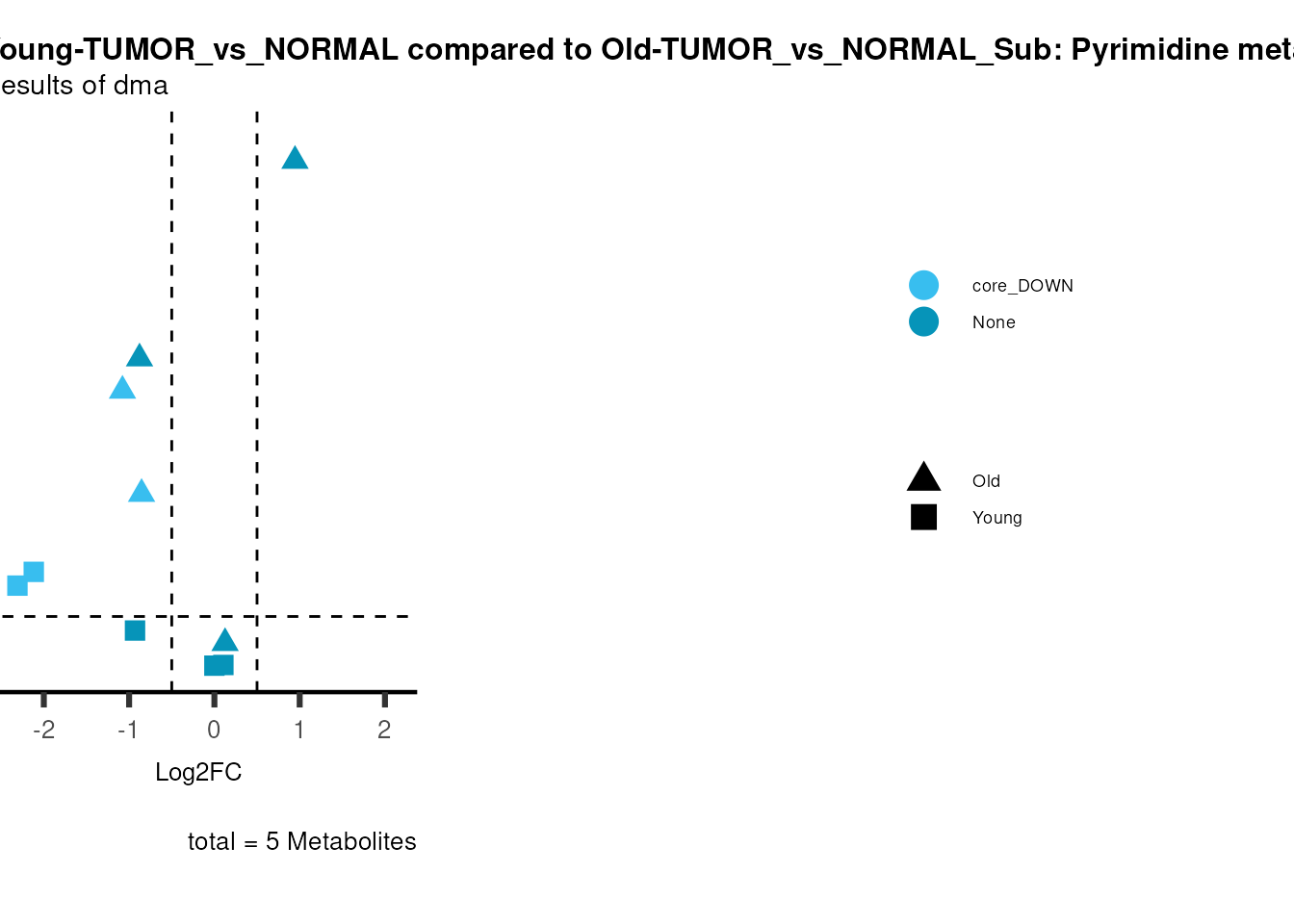
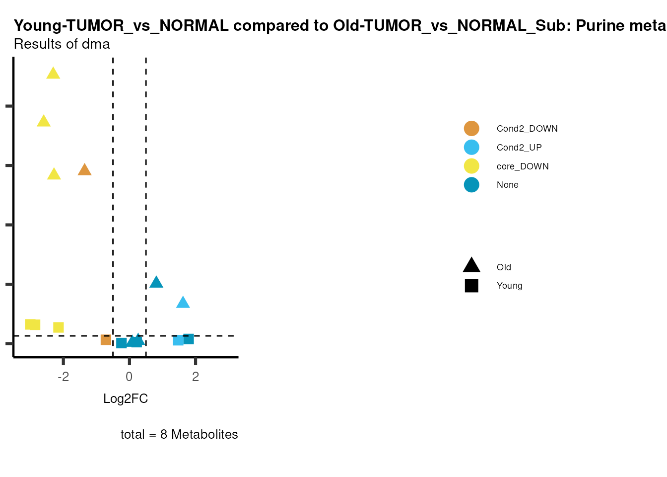
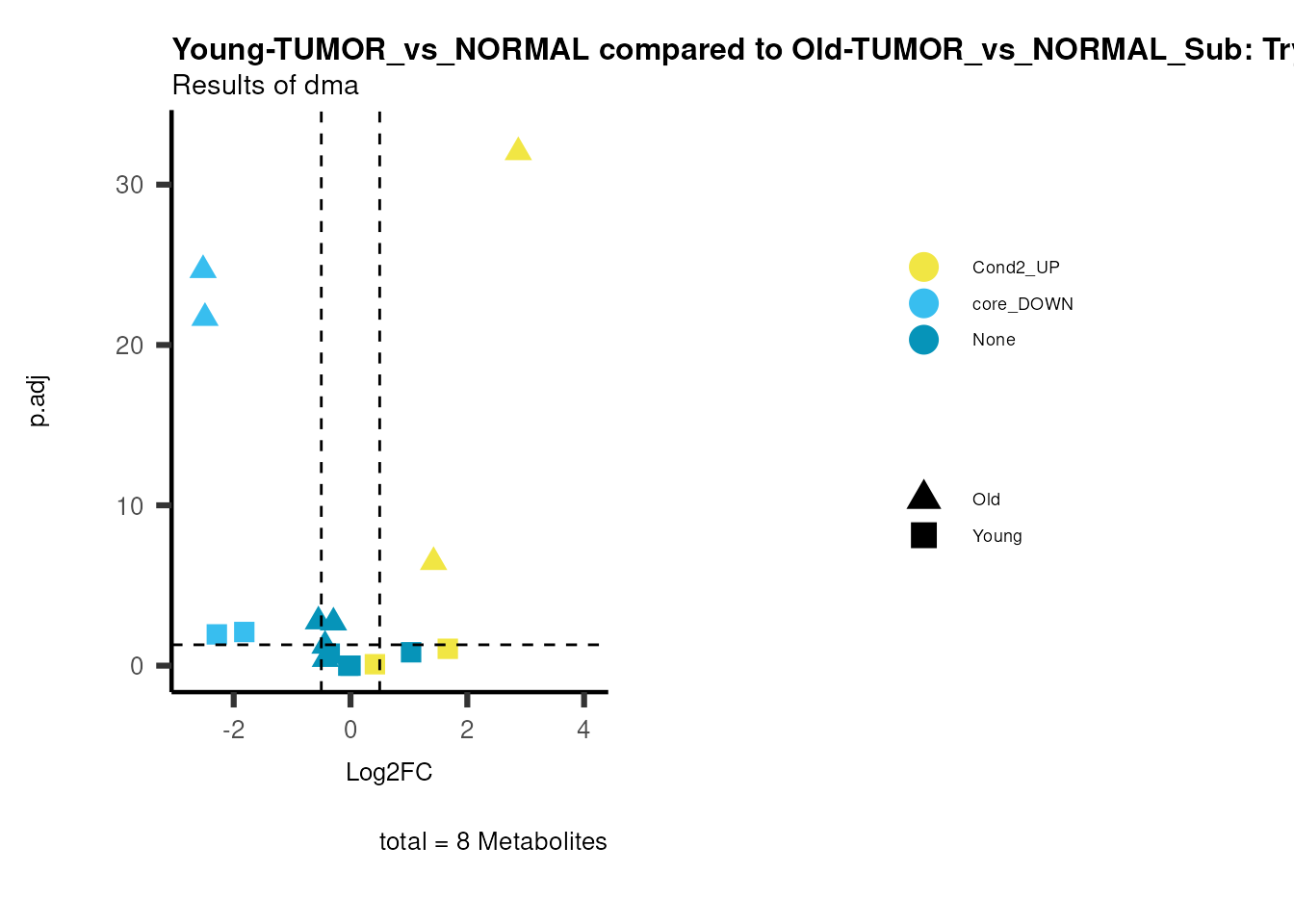
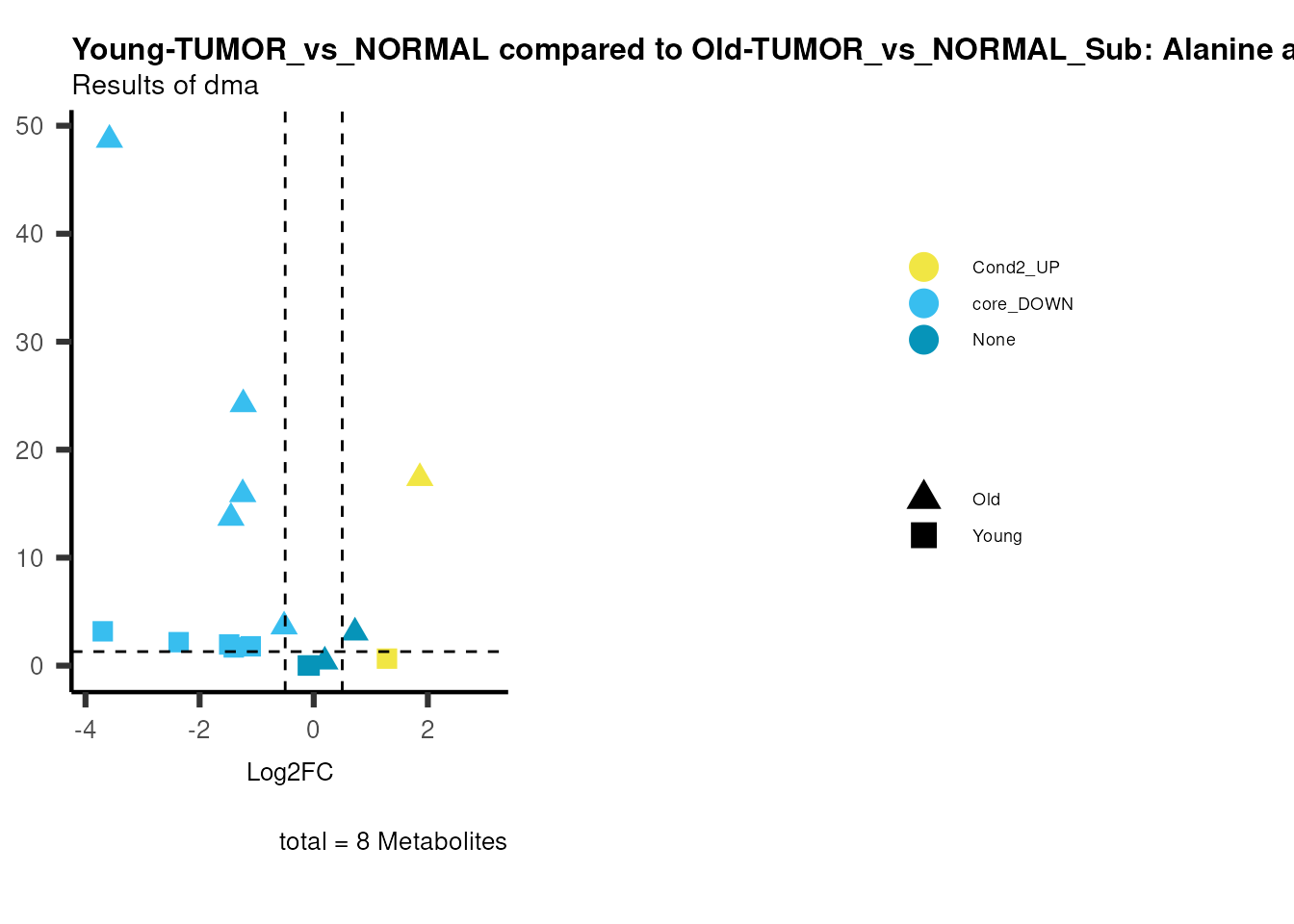
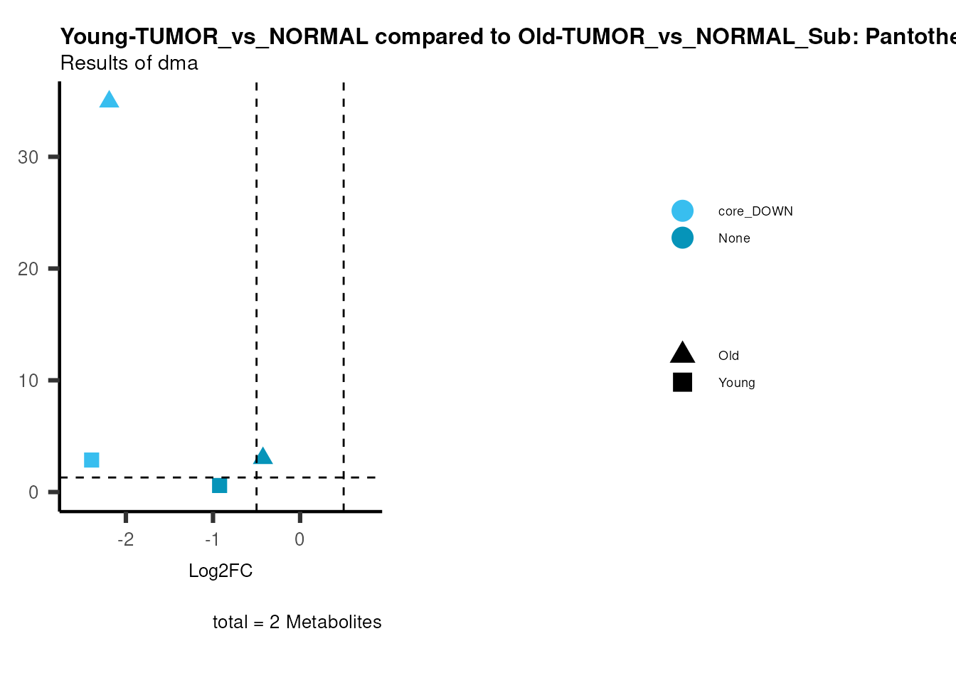
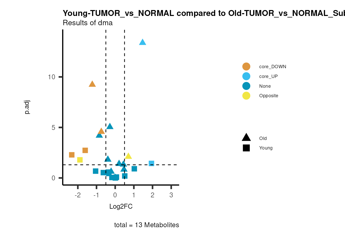
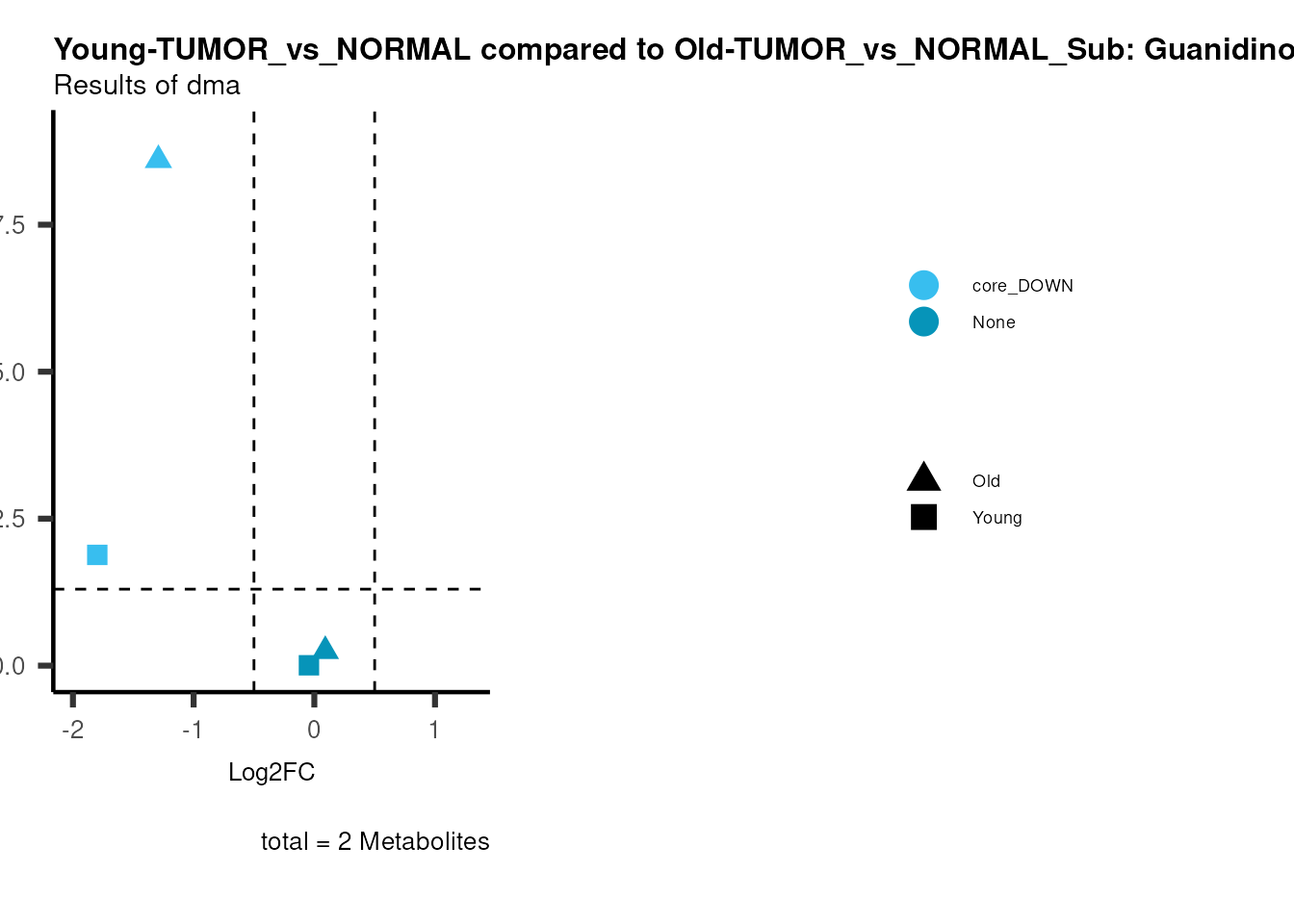
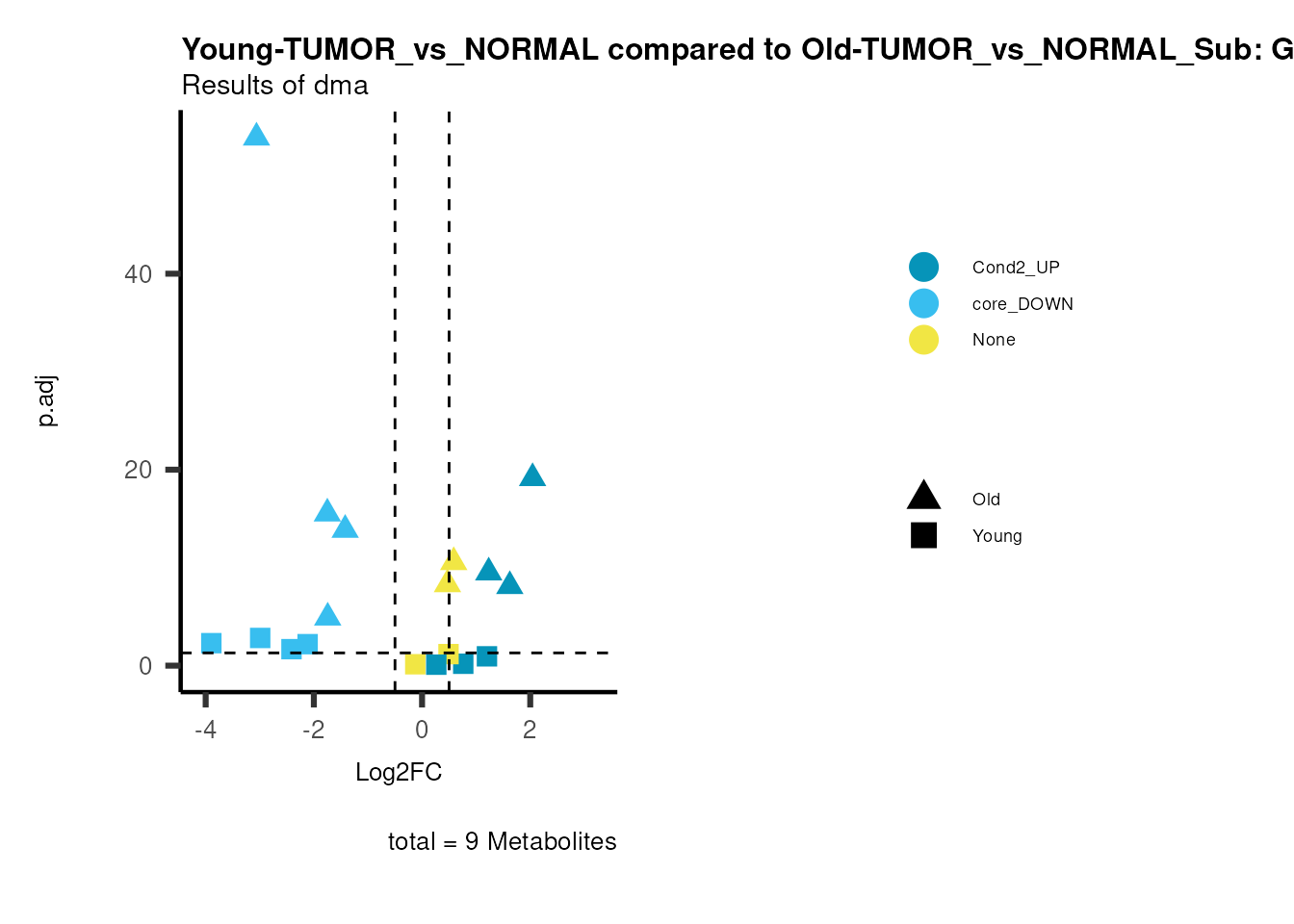
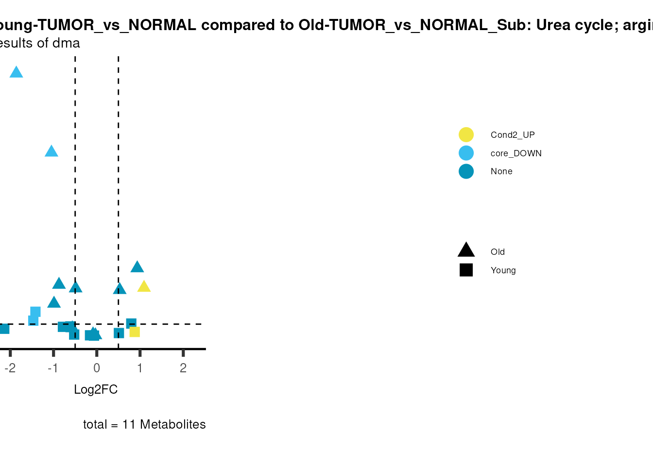
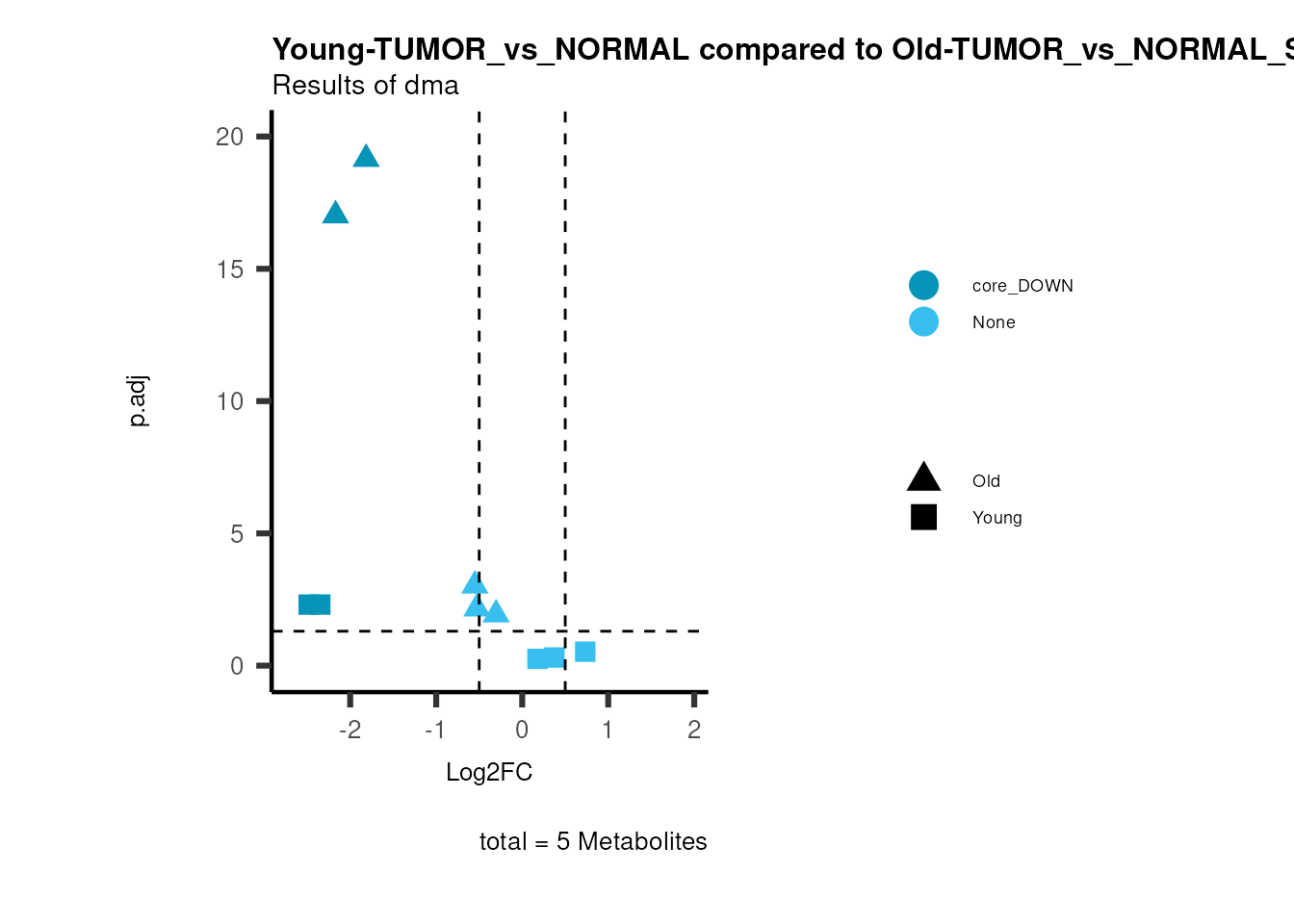
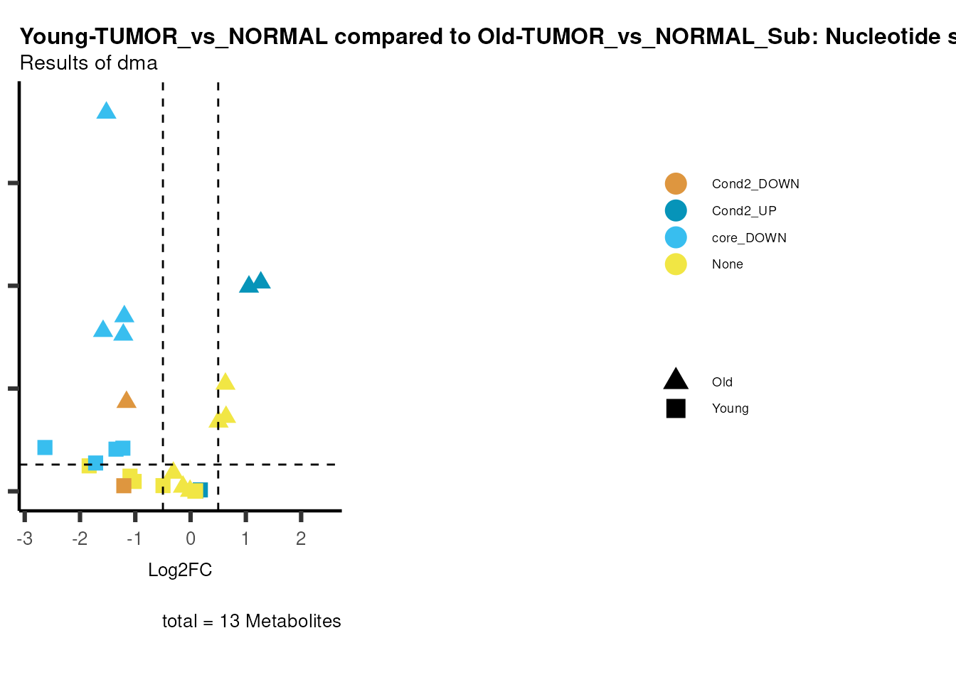
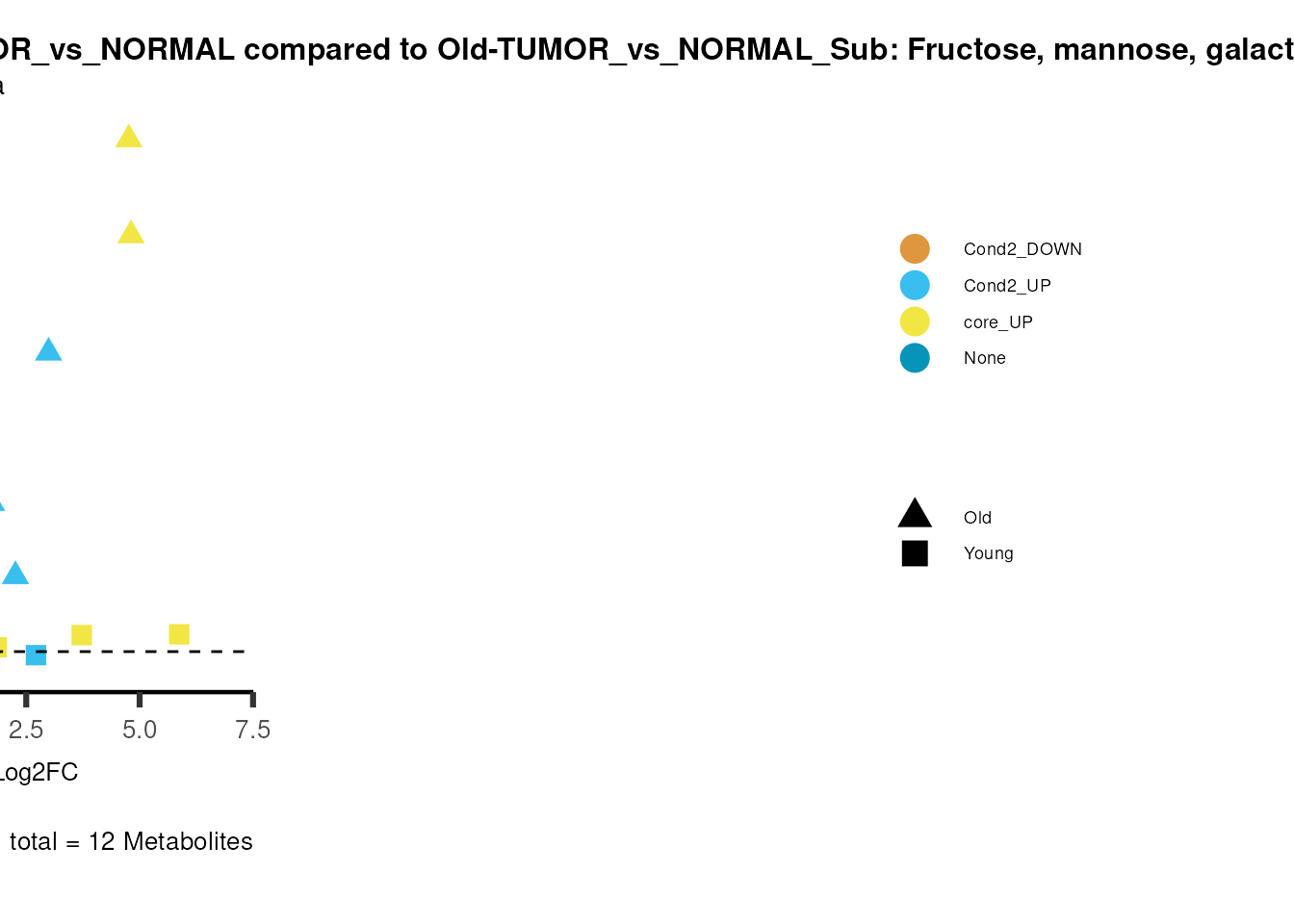
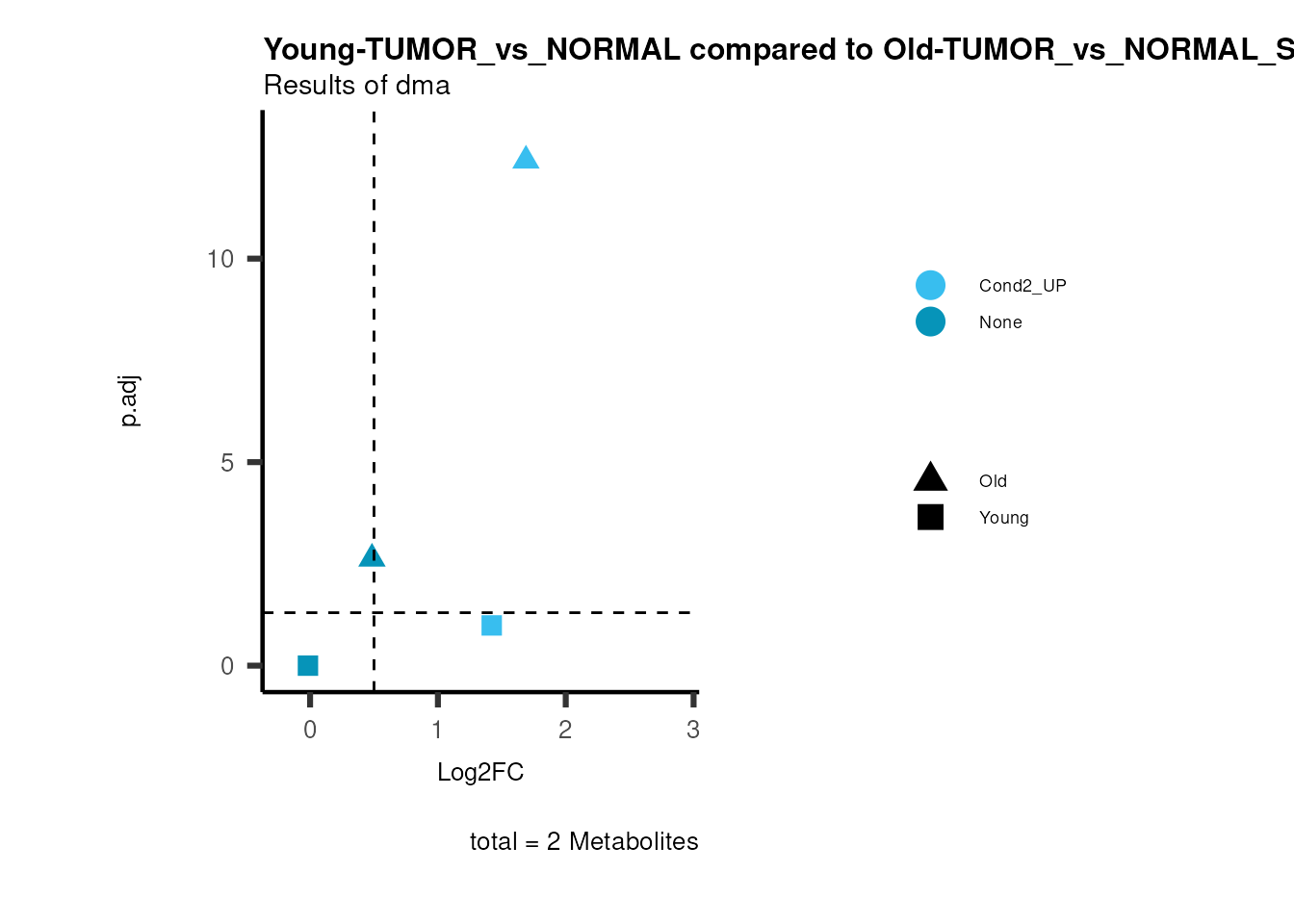
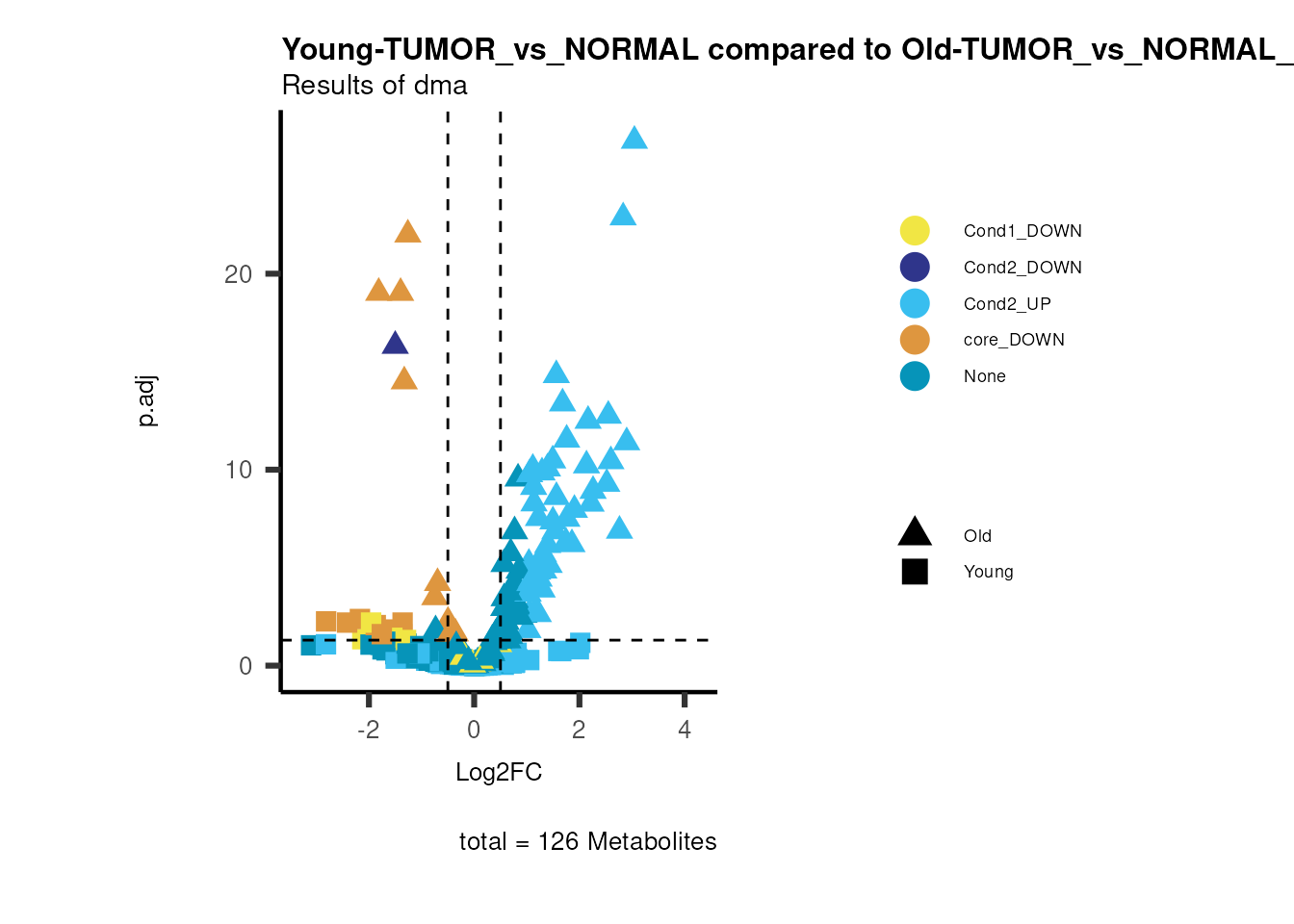
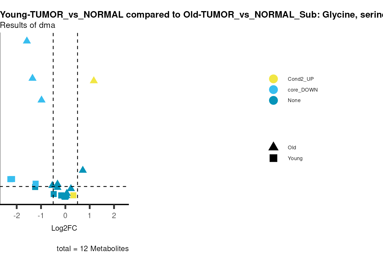
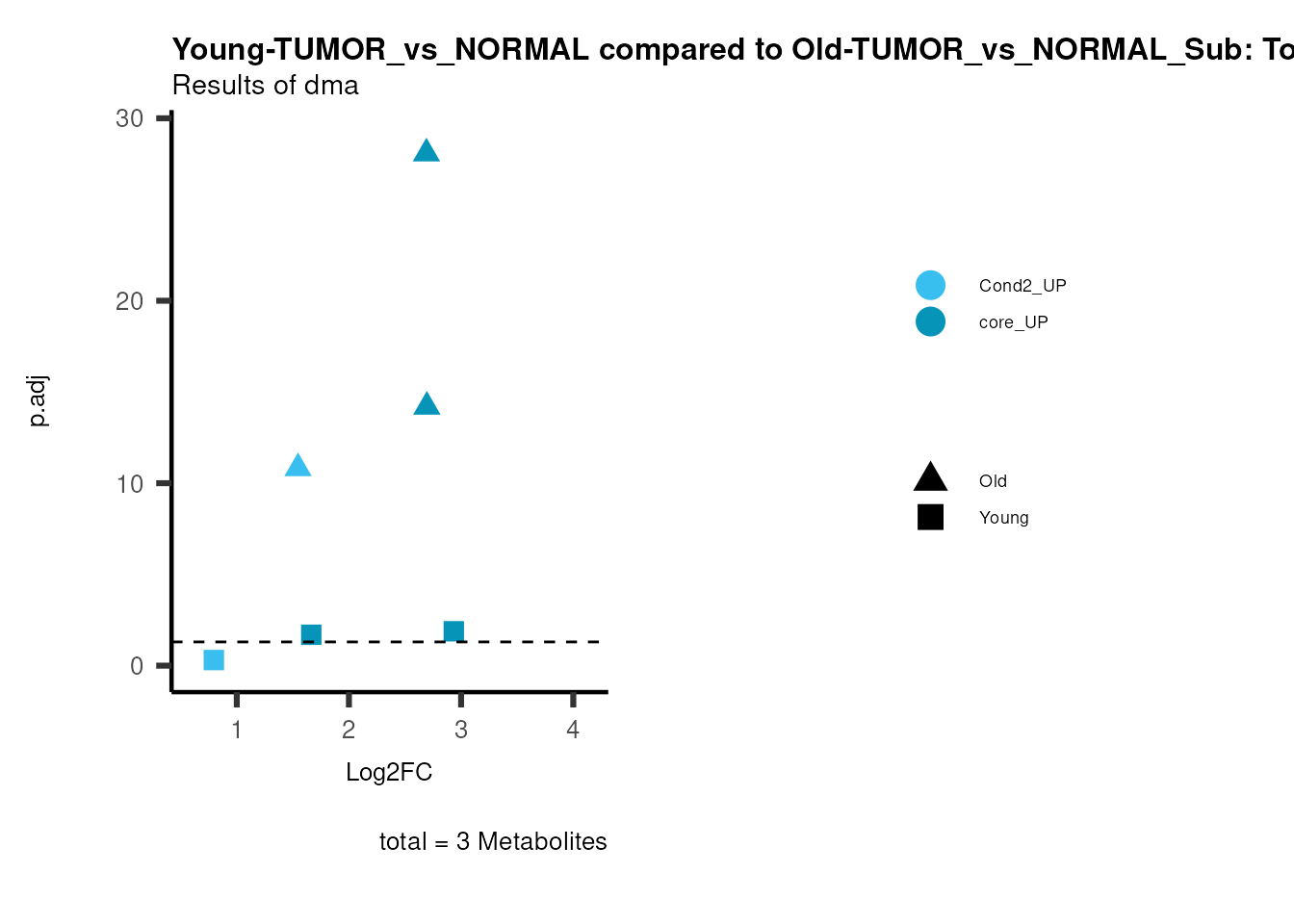
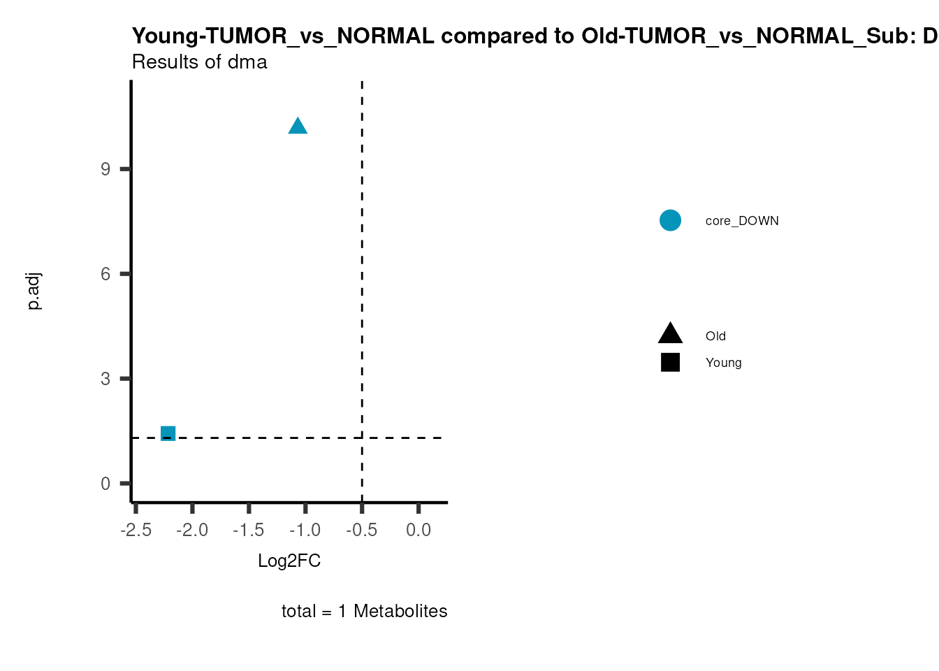
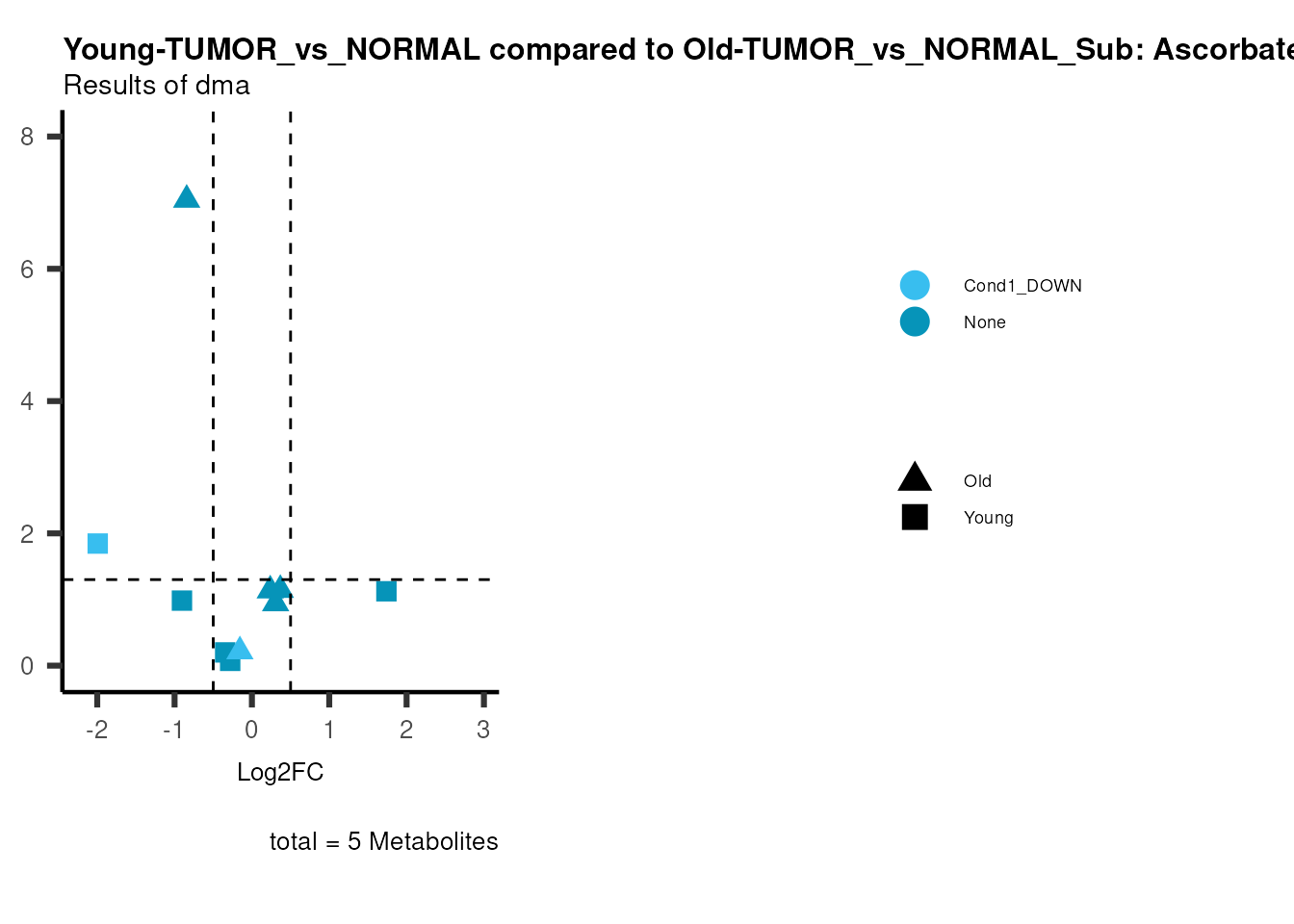
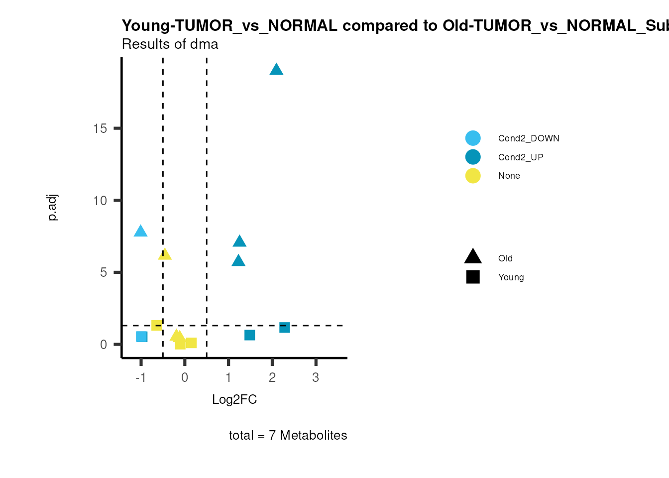
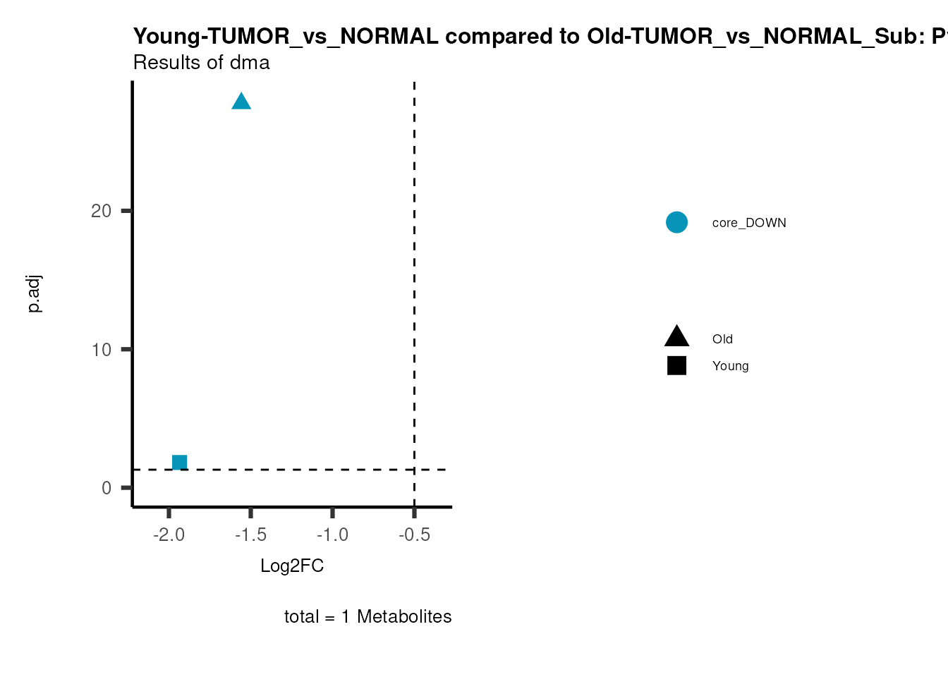
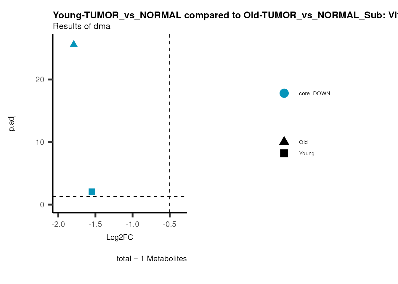
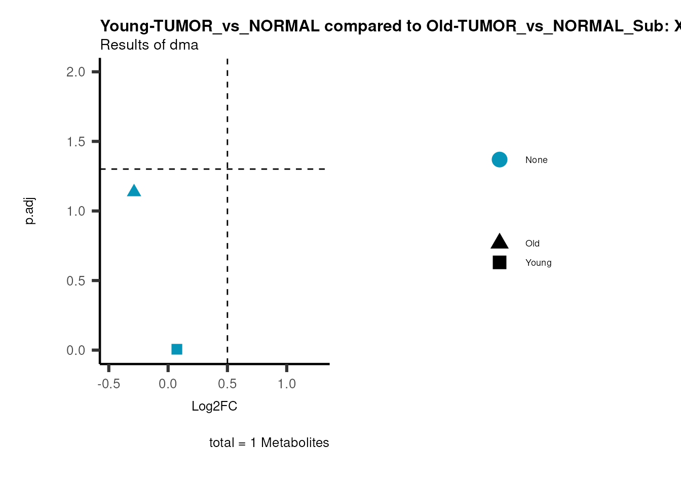
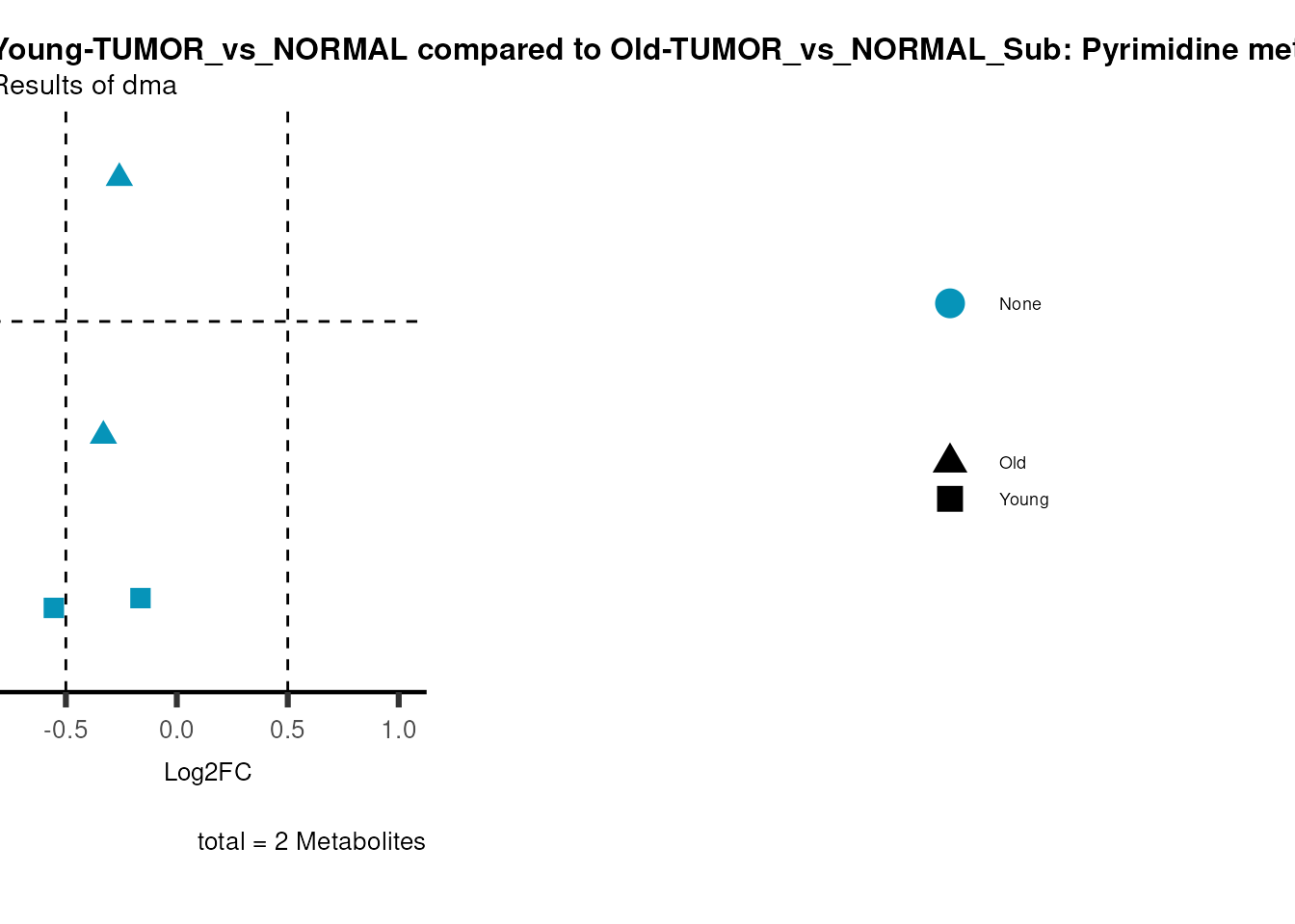
Now we can use this information to colour code our volcano plot. We will plot individual volcano plots for each metabolite pathway as defined by the feature metadata provided as part of the data in (Hakimi et al. 2016).

# Add metabolite information such as KEGG ID or pathway to results
MetaData_Metab <- merge(x=Tissue_MetaData,
y= MCAres[["MCA_2Cond_Results"]][, c(1, 14:15)],
by="Metabolite",
all.y=TRUE)%>%
dplyr::filter(!is.na(SUPER_PATHWAY))%>%
dplyr::filter(!is.na(SUB_PATHWAY))

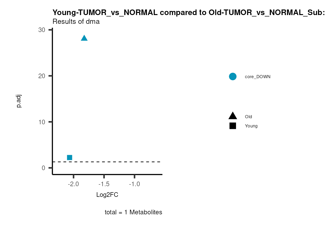
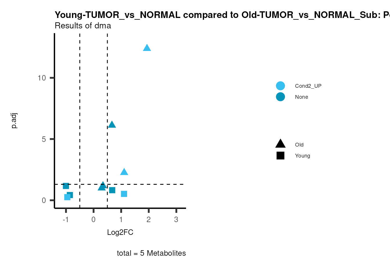
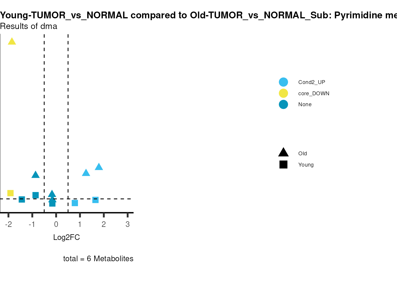
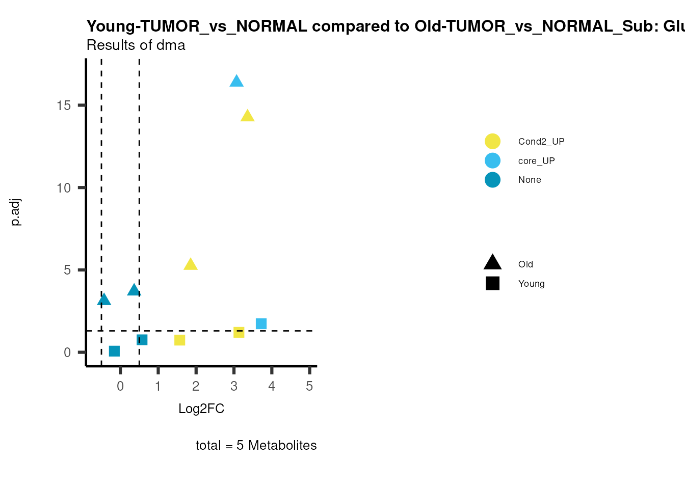
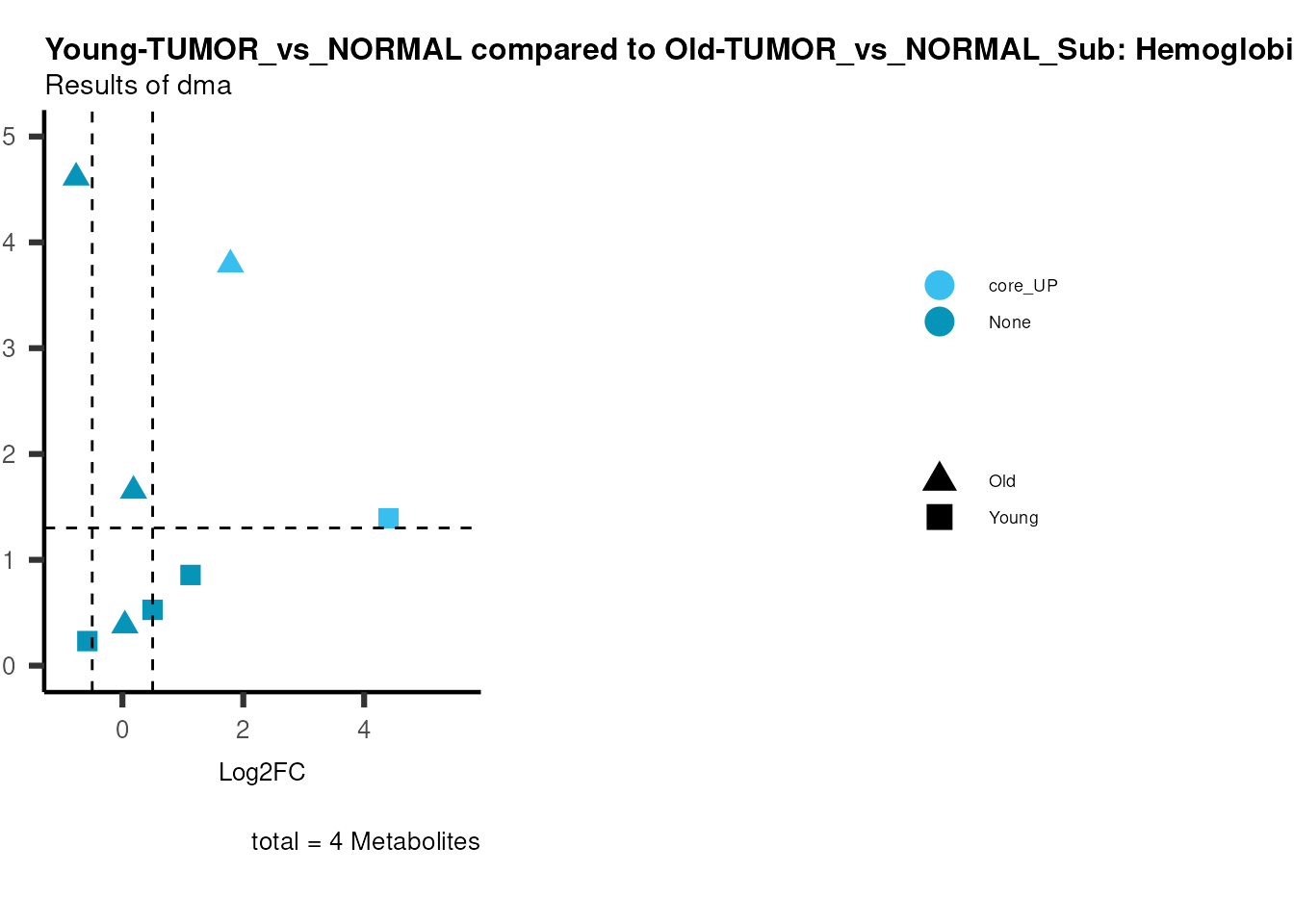
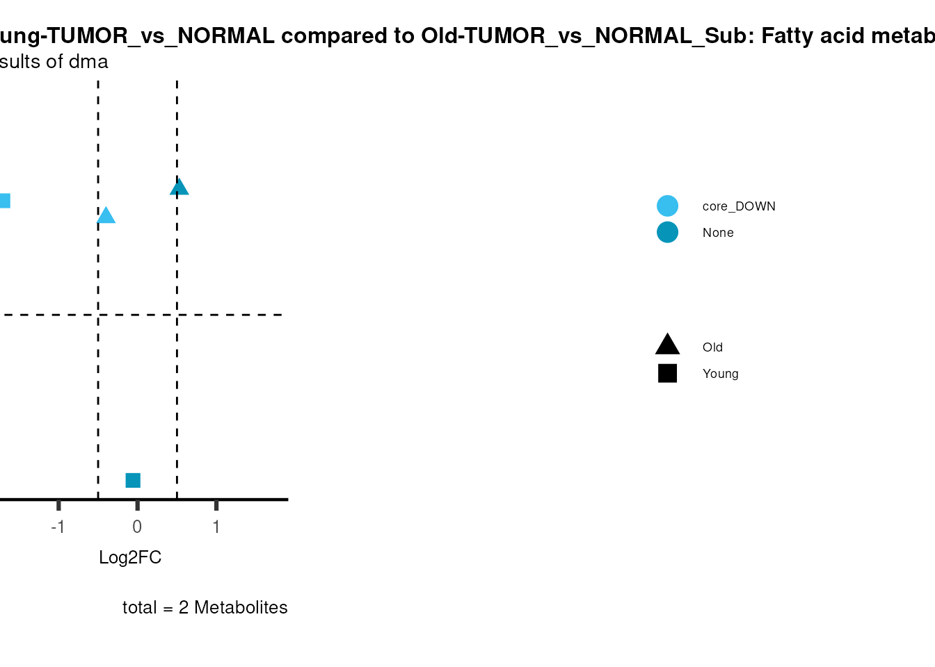
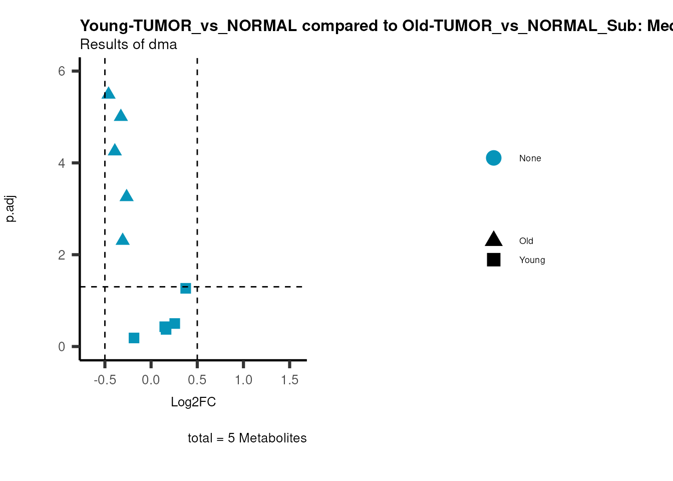
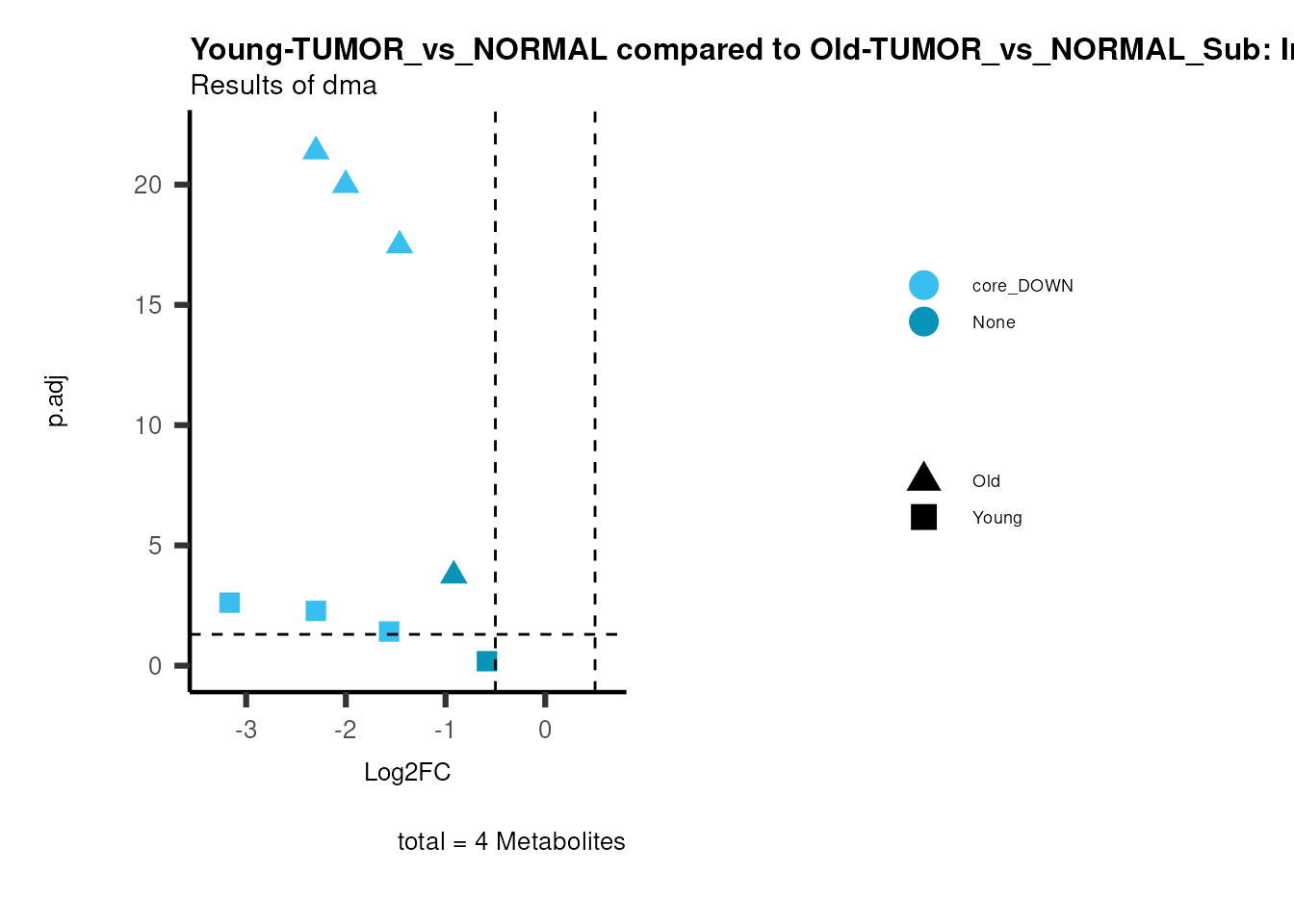
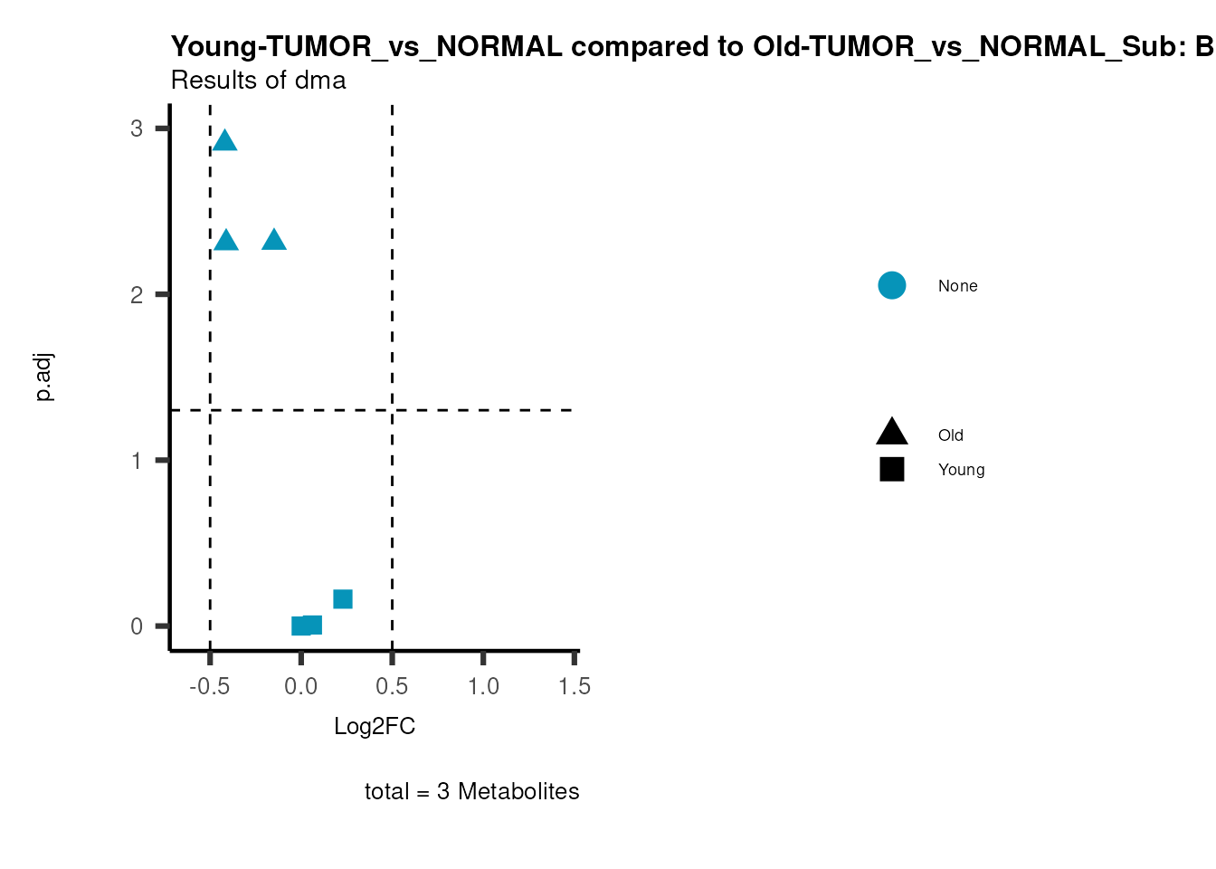
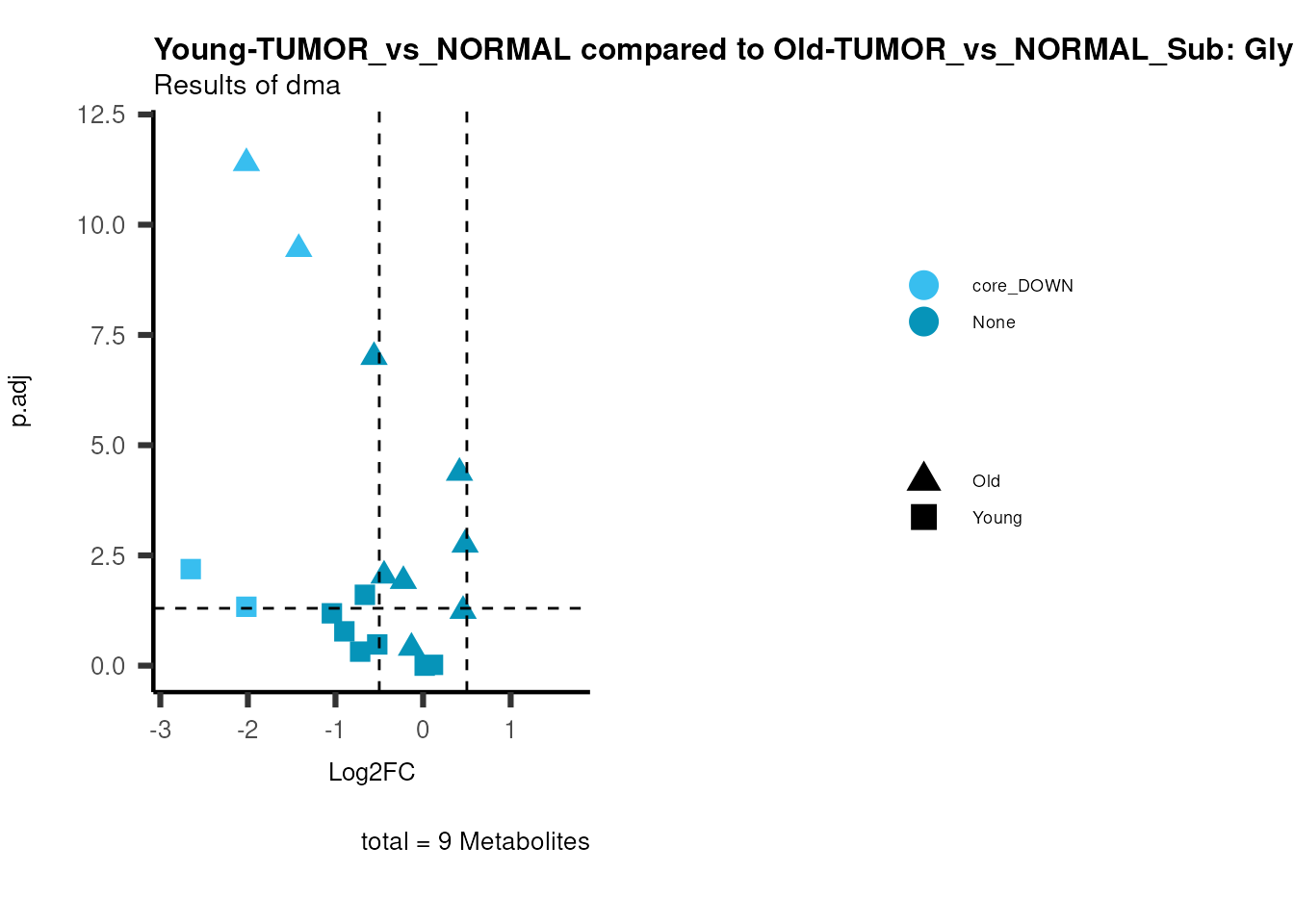
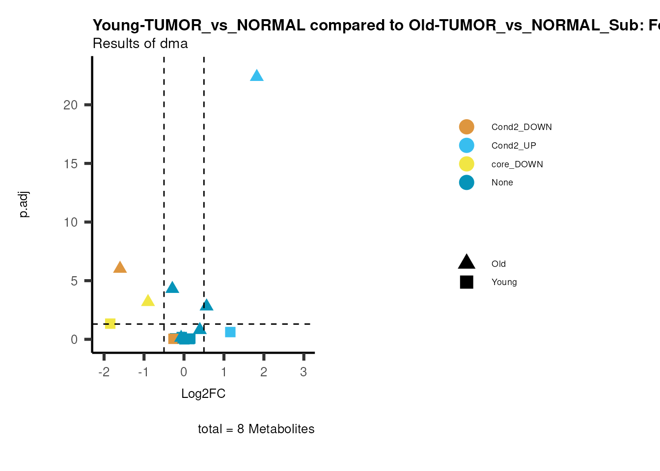
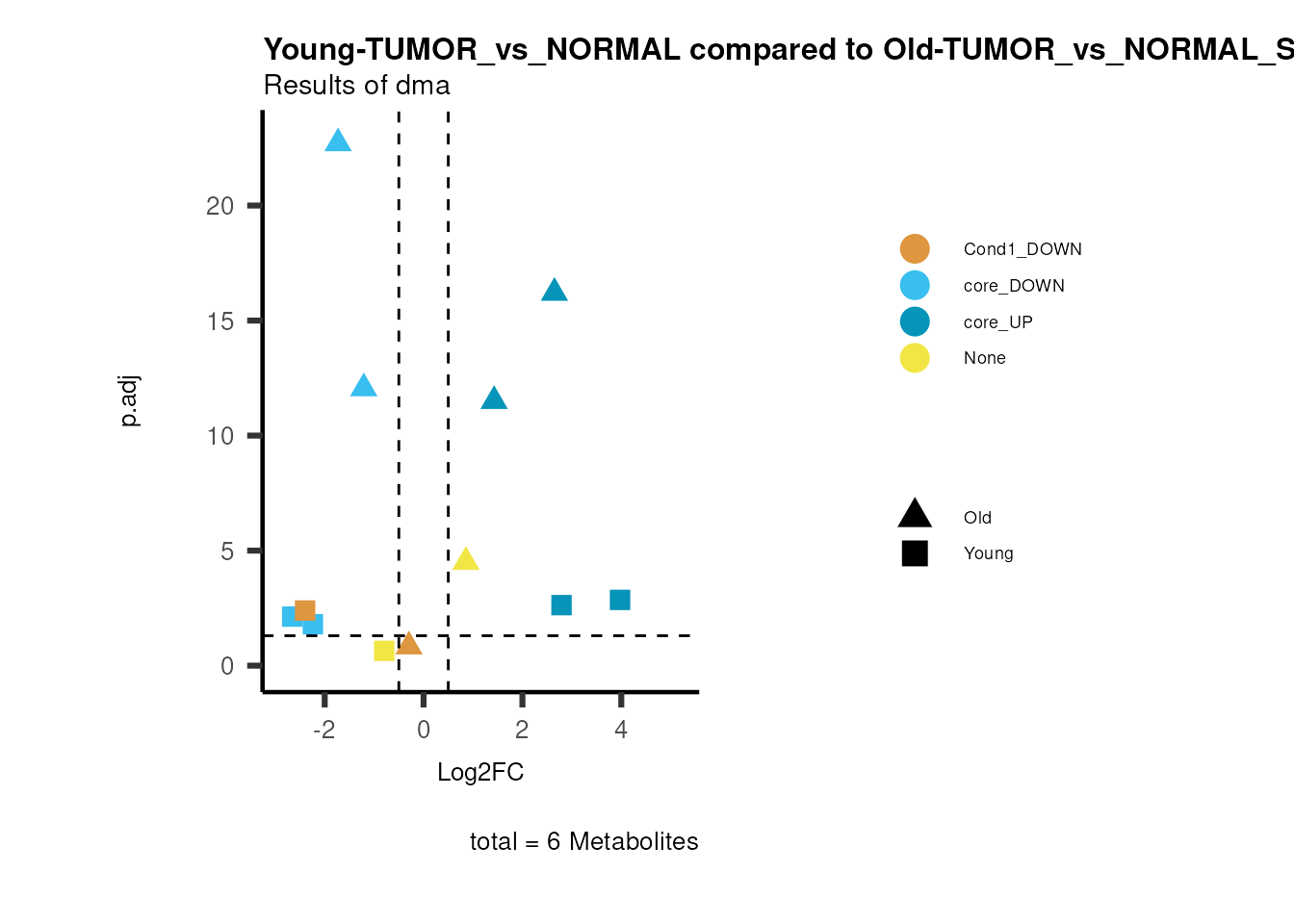
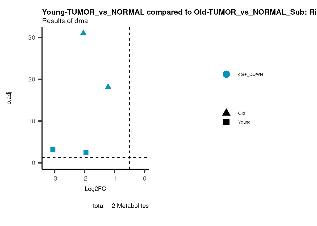
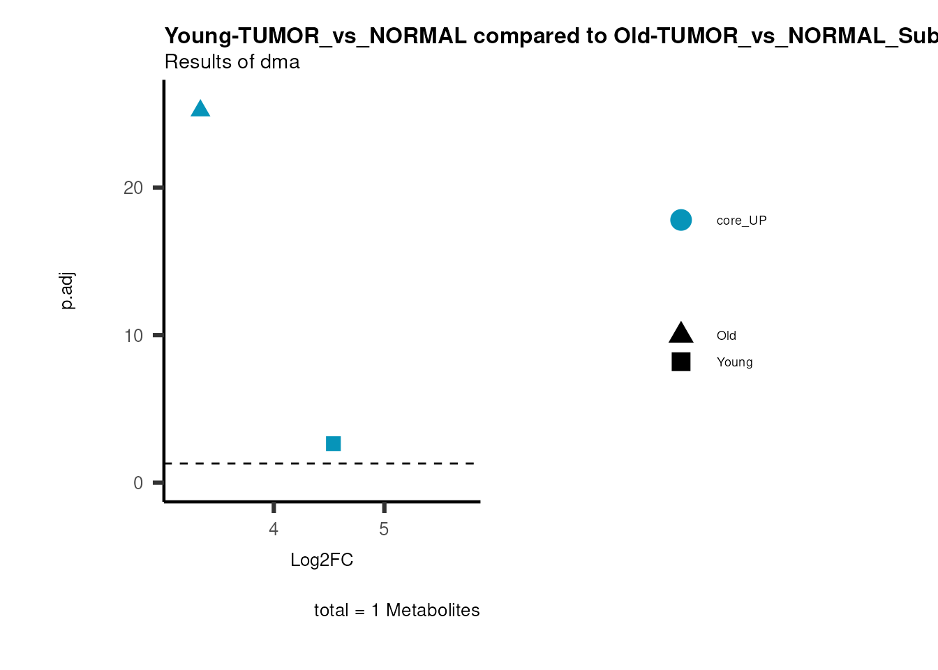
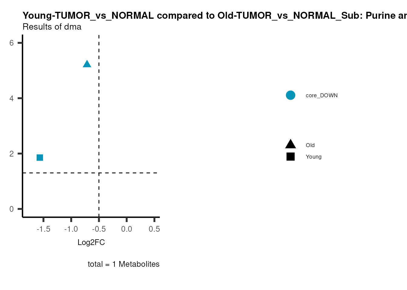
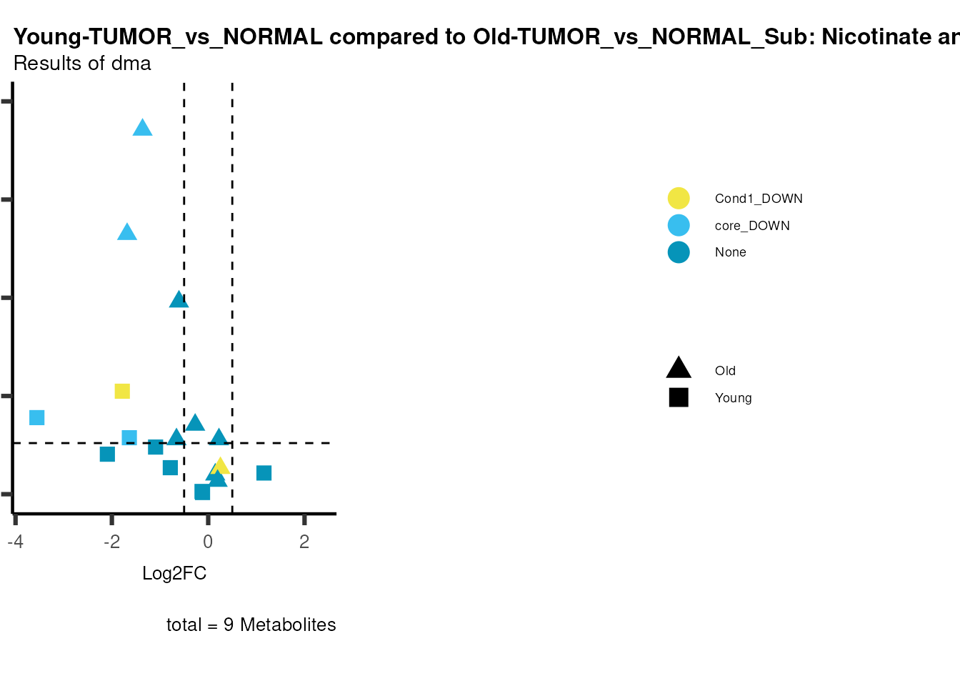
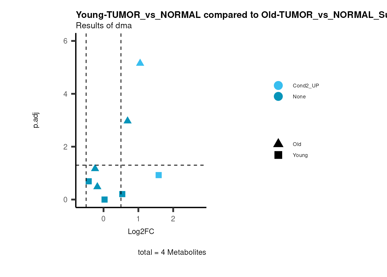
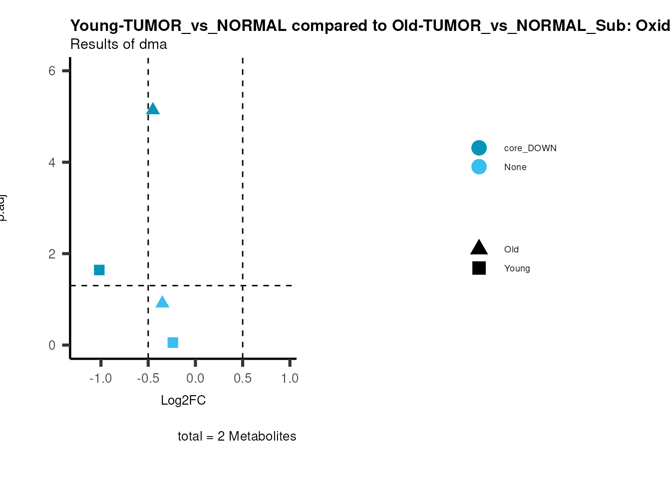
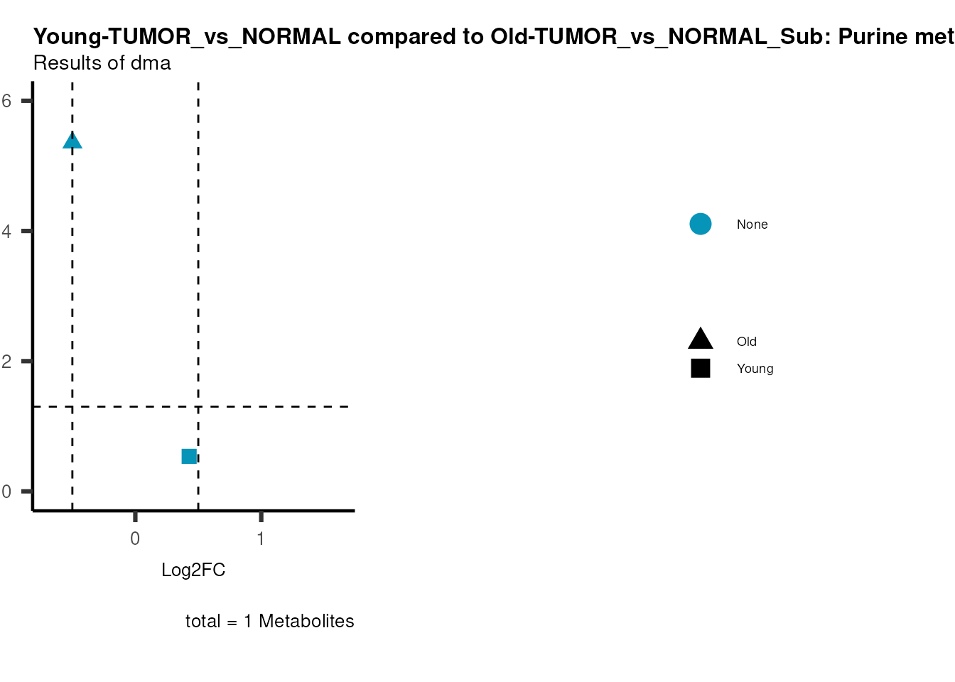
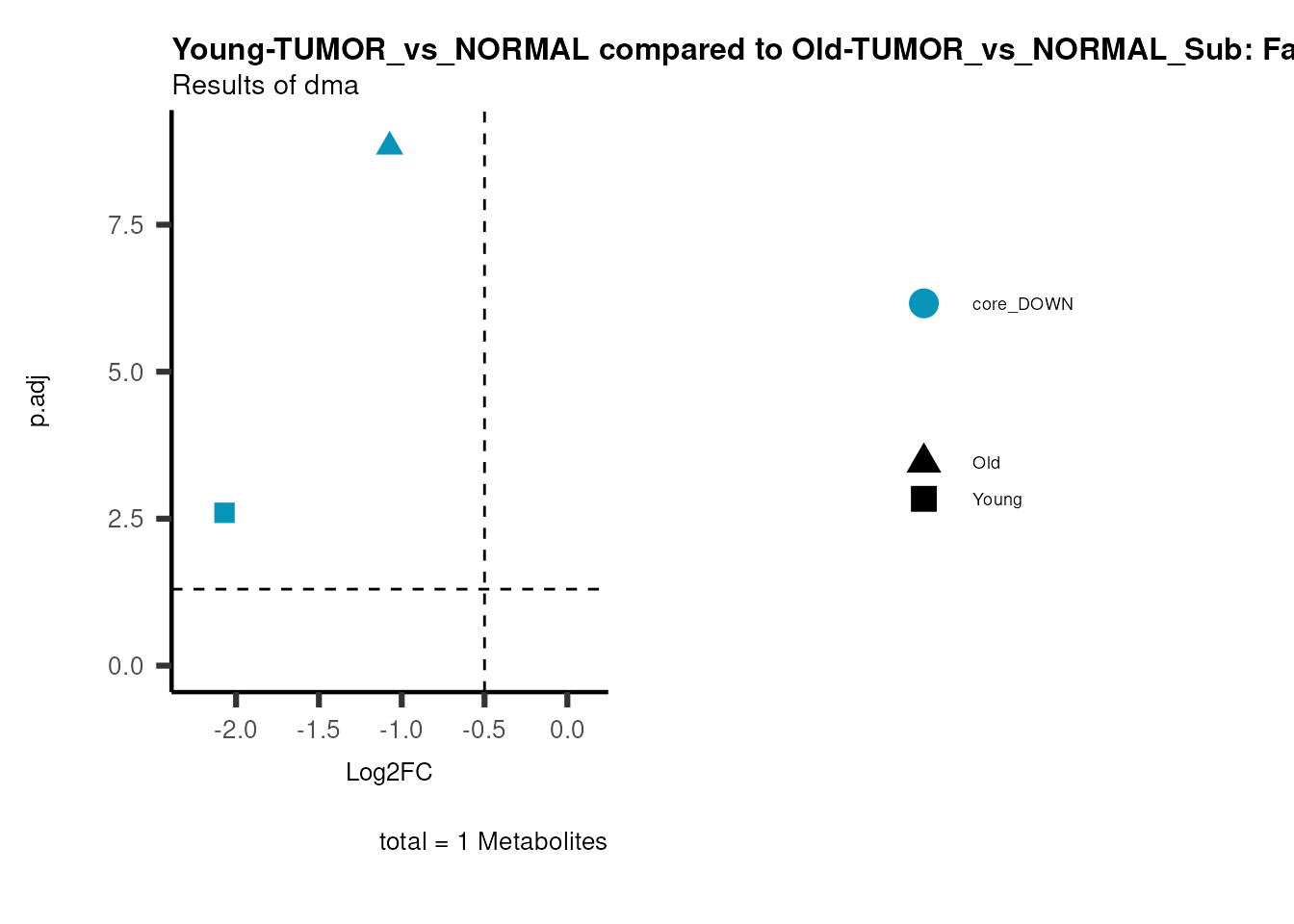
viz_volcano(plot_types="Compare",
data=ResList[["Young"]][["dma"]][["TUMOR_vs_NORMAL"]]%>%tibble::column_to_rownames("Metabolite"),
data2= ResList[["Old"]][["dma"]][["TUMOR_vs_NORMAL"]]%>%tibble::column_to_rownames("Metabolite"),
name_comparison= c(data="Young", data2= "Old"),
metadata_feature =  MetaData_Metab%>%tibble::column_to_rownames("Metabolite"),
plot_name= "Young-TUMOR_vs_NORMAL compared to Old-TUMOR_vs_NORMAL",
subtitle= "Results of dma",
metadata_info = c(individual = "SUPER_PATHWAY",
                                        color = "RG2_Significant"))

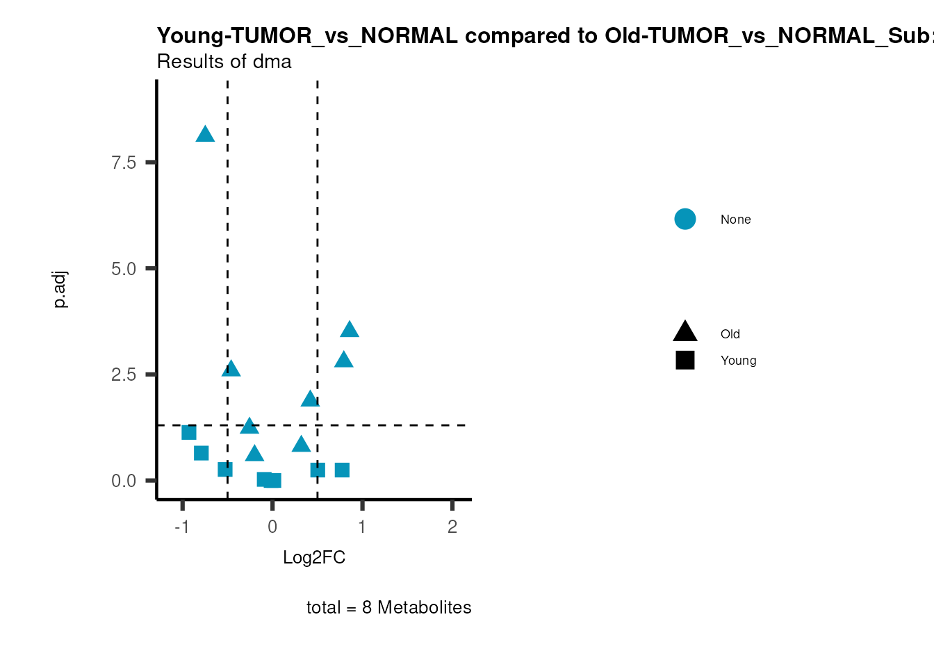
viz_volcano(plot_types="Compare",
data=ResList[["Young"]][["dma"]][["TUMOR_vs_NORMAL"]]%>%tibble::column_to_rownames("Metabolite"),
data2= ResList[["Old"]][["dma"]][["TUMOR_vs_NORMAL"]]%>%tibble::column_to_rownames("Metabolite"),
name_comparison= c(data="Young", data2= "Old"),
metadata_feature =  MetaData_Metab%>%tibble::column_to_rownames("Metabolite"),
plot_name= "Young-TUMOR_vs_NORMAL compared to Old-TUMOR_vs_NORMAL_Sub",
subtitle= "Results of dma",
metadata_info = c(individual = "SUB_PATHWAY",
                                        color = "RG2_Significant"))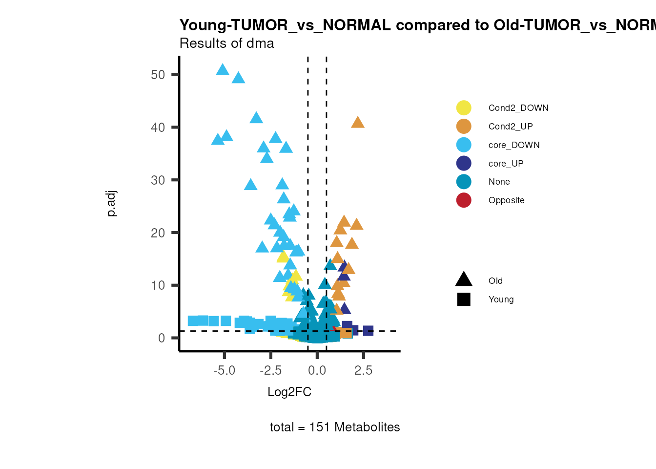

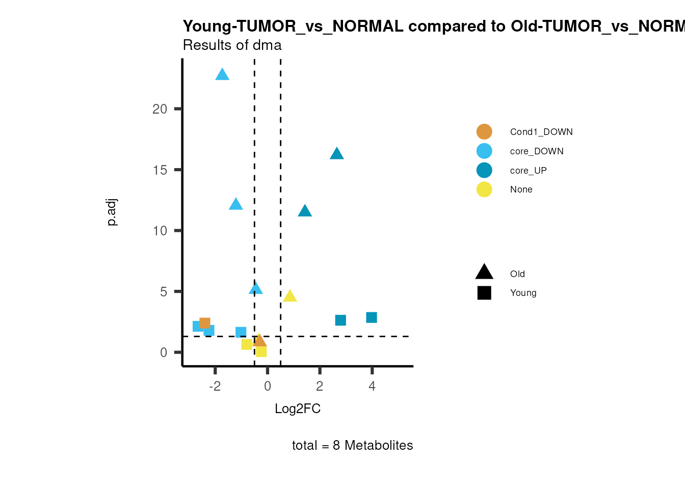
#> Skipping viz_volcano compare plot for 'NA' because no rows are available after filtering.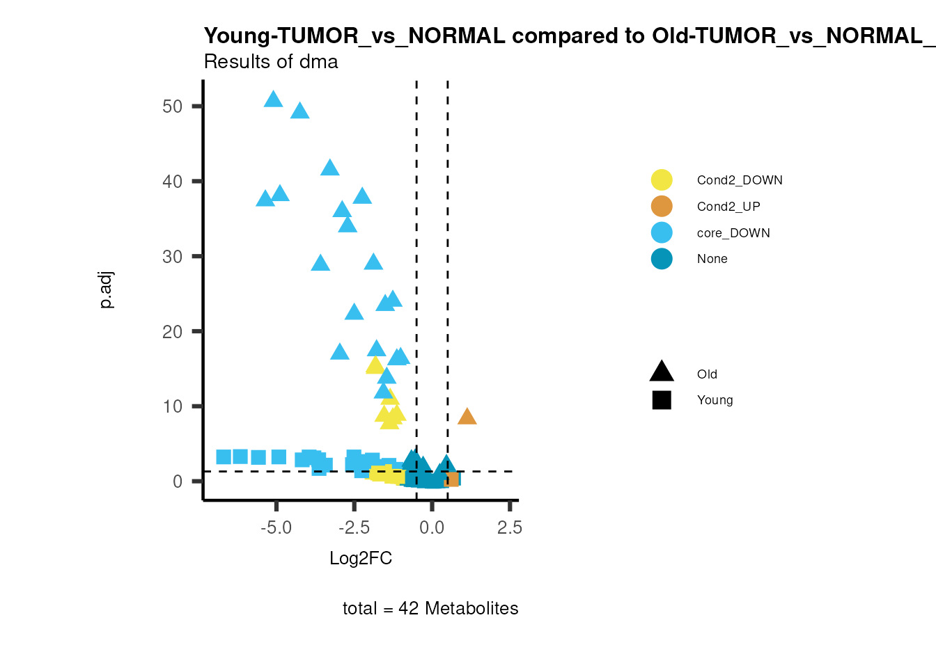

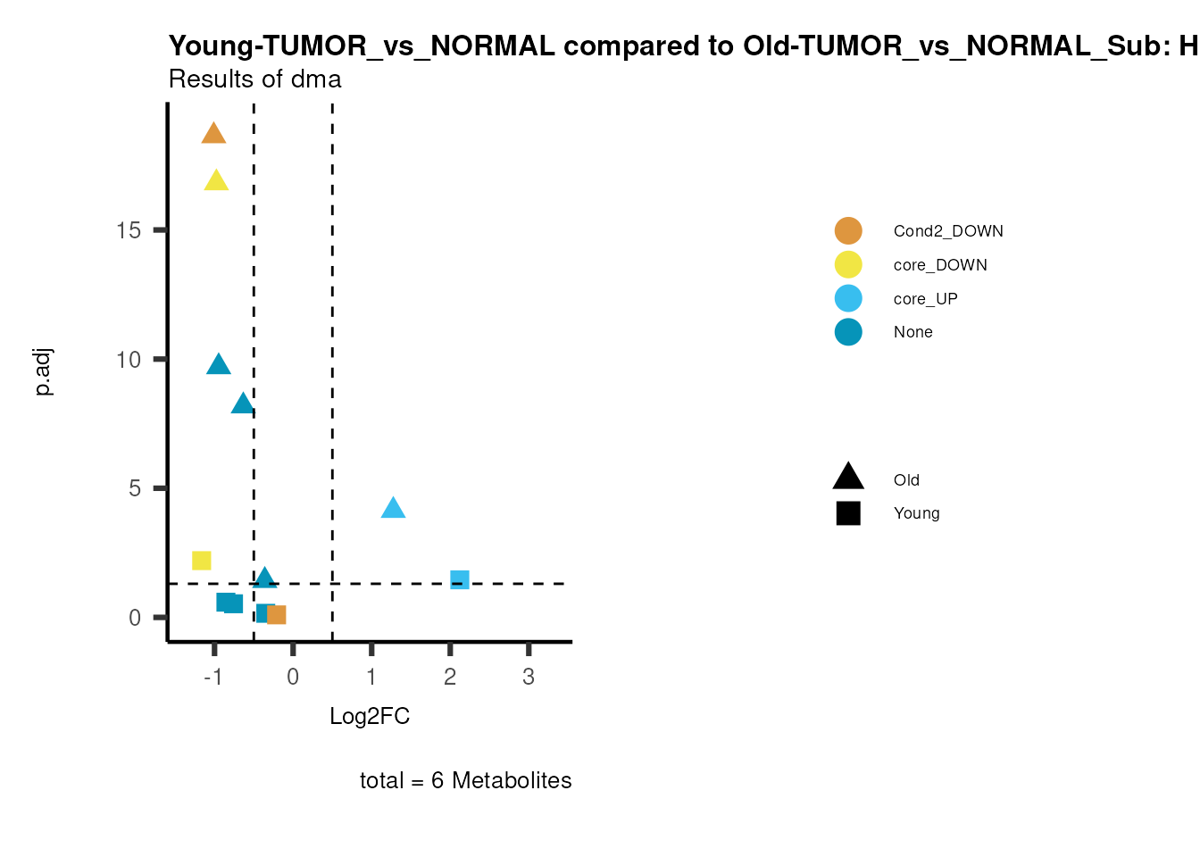
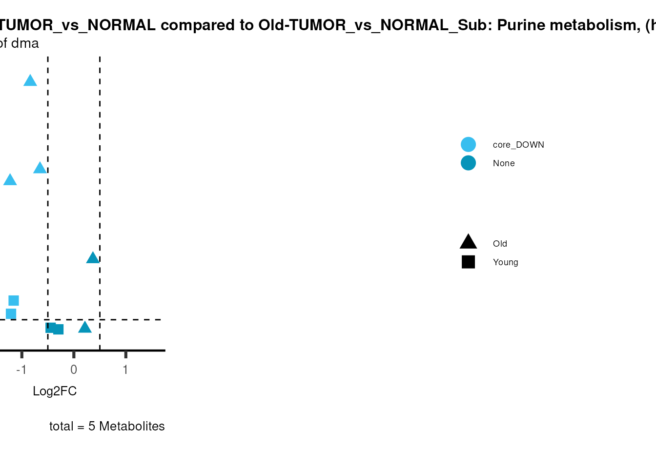
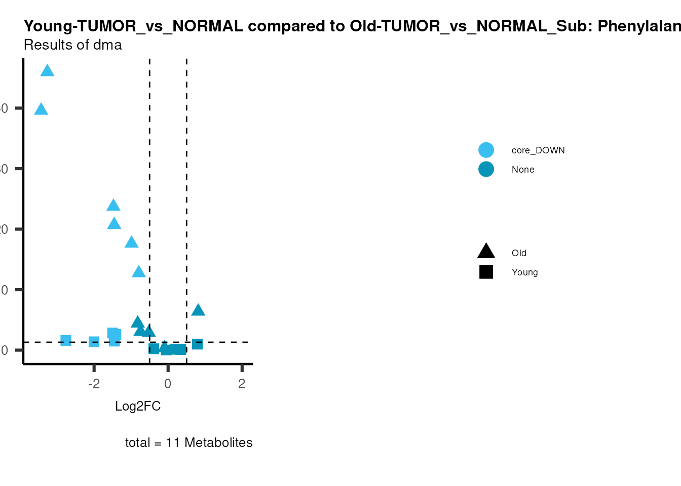
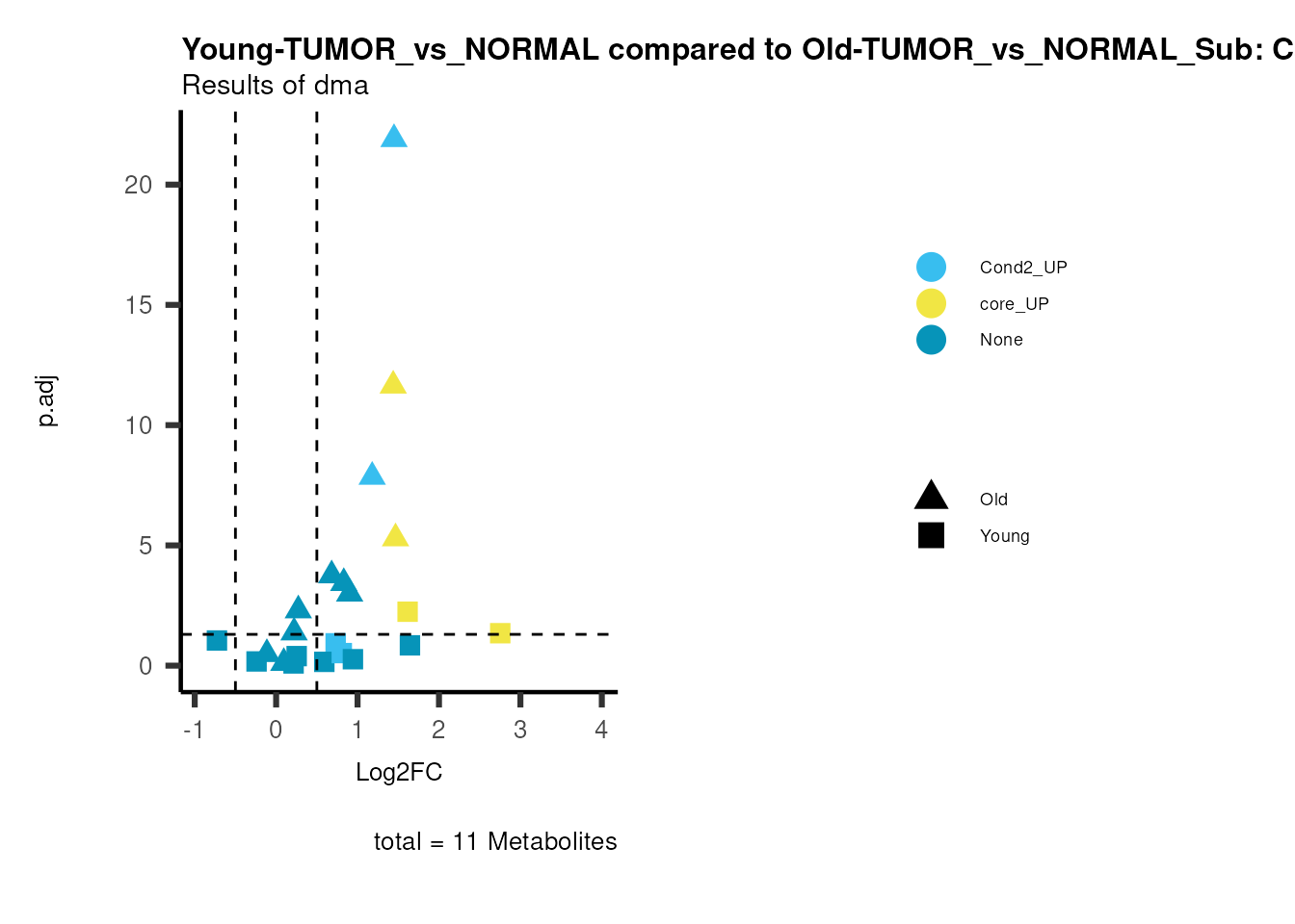
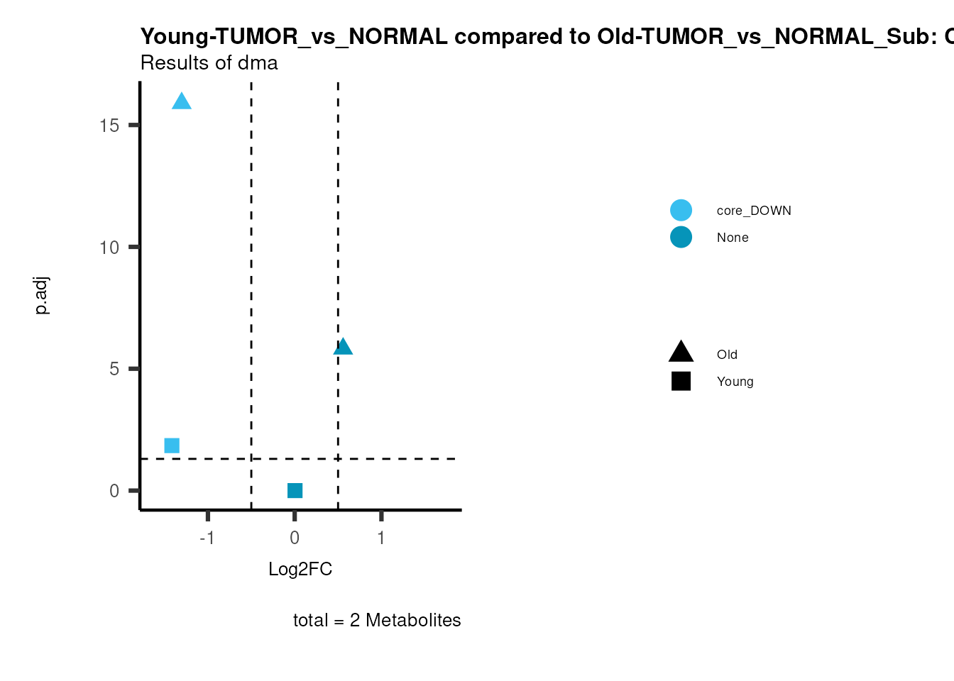
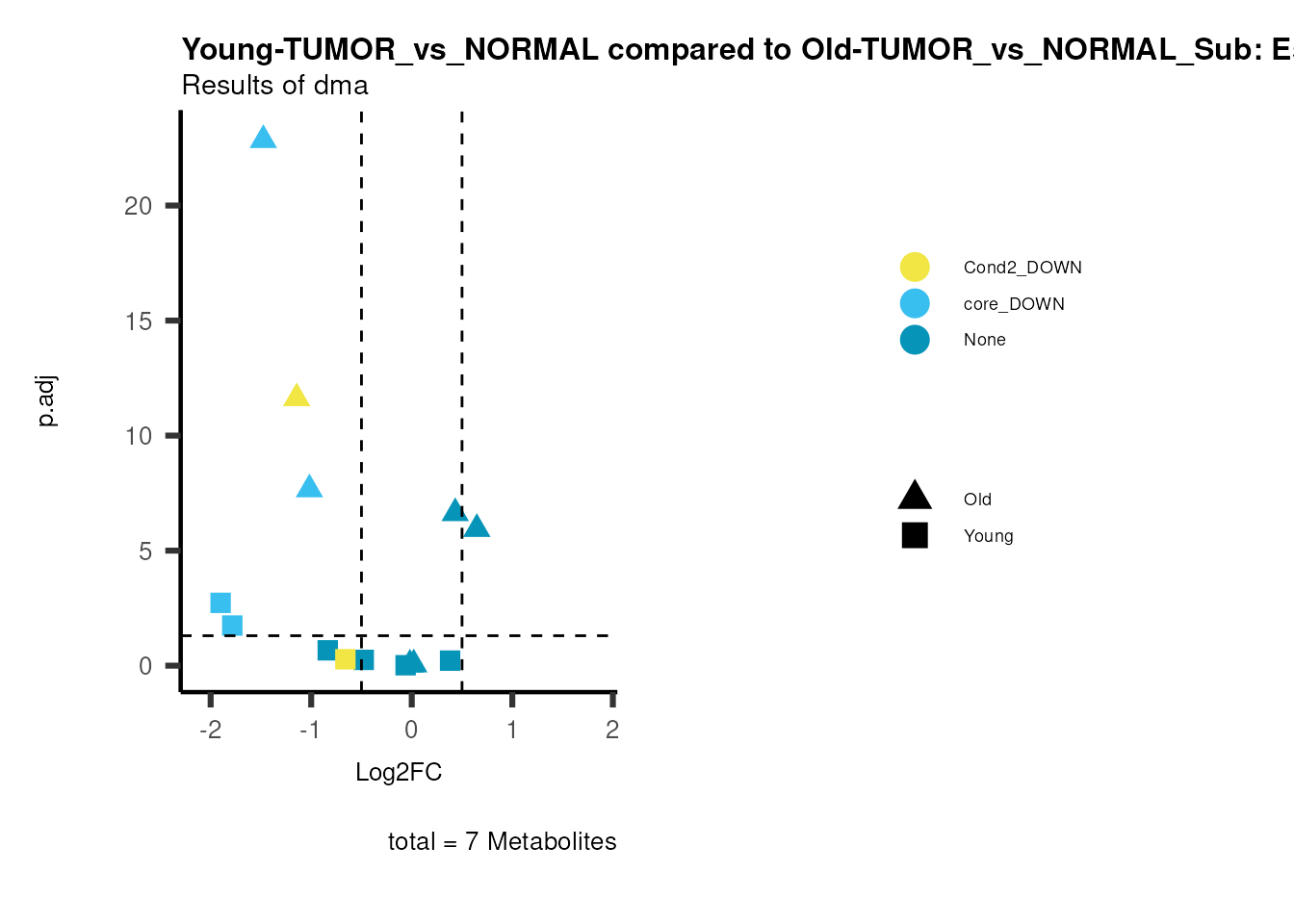
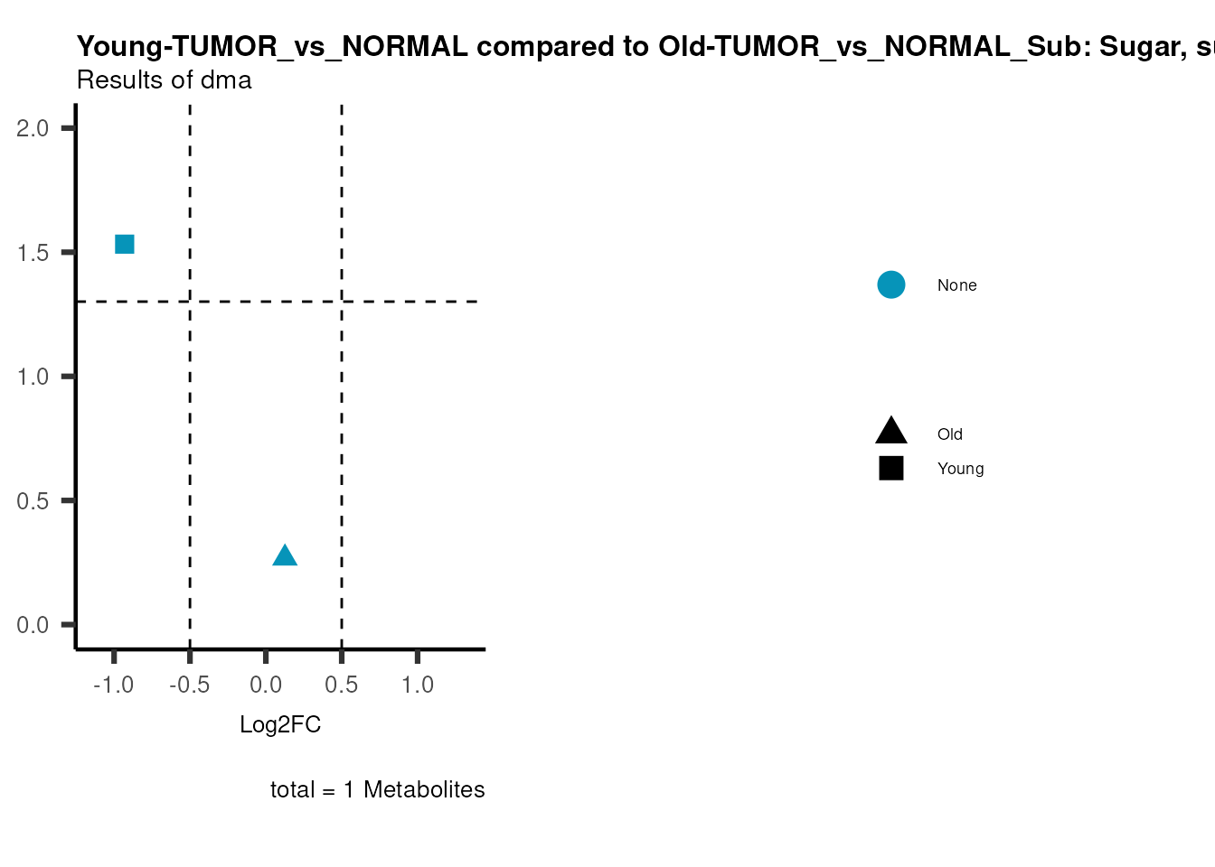
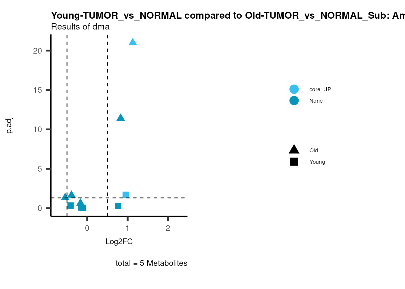
#> Skipping viz_volcano compare plot for 'NA' because no rows are available after filtering.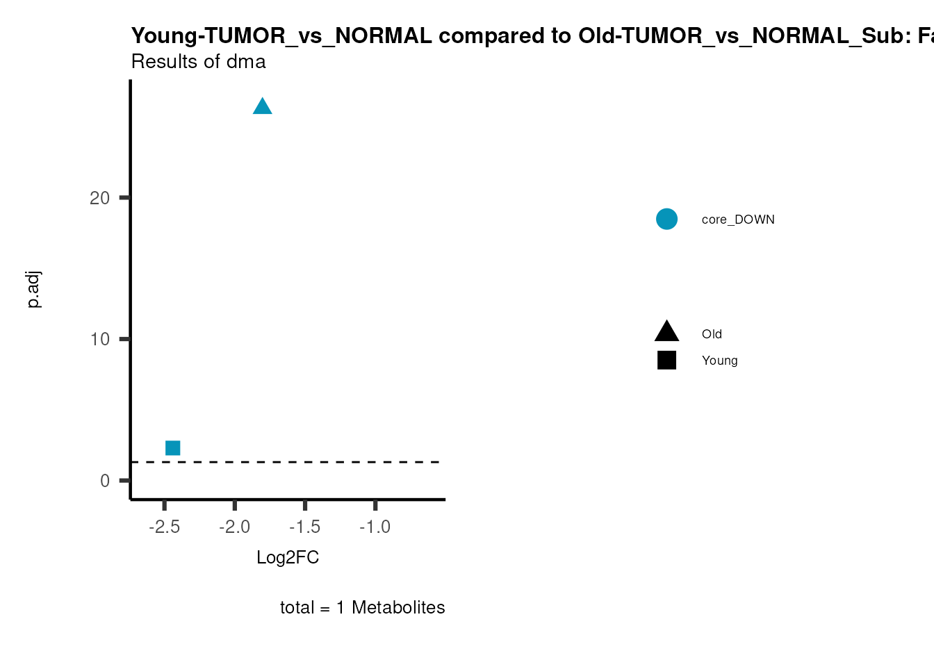

Session information

#> R version 4.6.1 (2026-06-24)
#> Platform: x86_64-pc-linux-gnu
#> Running under: Ubuntu 24.04.4 LTS
#> 
#> Matrix products: default
#> BLAS:   /usr/lib/x86_64-linux-gnu/openblas-pthread/libblas.so.3 
#> LAPACK: /usr/lib/x86_64-linux-gnu/openblas-pthread/libopenblasp-r0.3.26.so;  LAPACK version 3.12.0
#> 
#> locale:
#>  [1] LC_CTYPE=en_US.UTF-8       LC_NUMERIC=C               LC_TIME=en_US.UTF-8        LC_COLLATE=en_US.UTF-8    
#>  [5] LC_MONETARY=en_US.UTF-8    LC_MESSAGES=en_US.UTF-8    LC_PAPER=en_US.UTF-8       LC_NAME=C                 
#>  [9] LC_ADDRESS=C               LC_TELEPHONE=C             LC_MEASUREMENT=en_US.UTF-8 LC_IDENTIFICATION=C       
#> 
#> time zone: Etc/UTC
#> tzcode source: system (glibc)
#> 
#> attached base packages:
#> [1] stats     graphics  grDevices utils     datasets  methods   base     
#> 
#> other attached packages:
#> [1] stringr_1.6.0     tibble_3.3.1      tidyr_1.3.2       rlang_1.3.0       dplyr_1.2.1       magrittr_2.0.5   
#> [7] MetaProViz_4.99.0 BiocStyle_2.40.0 
#> 
#> loaded via a namespace (and not attached):
#>   [1] splines_4.6.1               later_1.4.8                 R.oo_1.27.1                 cellranger_1.1.0           
#>   [5] polyclip_1.10-7             XML_3.99-0.25               factoextra_2.2.0            lifecycle_1.0.5            
#>   [9] httr2_1.3.0                 tcltk_4.6.1                 rstatix_1.1.0               lattice_0.22-9             
#>  [13] vroom_1.7.1                 MASS_7.3-66                 backports_1.5.1             limma_3.68.5               
#>  [17] sass_0.4.10                 rmarkdown_2.32              jquerylib_0.1.4             yaml_2.3.12                
#>  [21] otel_0.2.0                  zip_3.0.2                   sessioninfo_1.2.4           EnhancedVolcano_1.31.0     
#>  [25] DBI_1.3.0                   RColorBrewer_1.1-3          lubridate_1.9.5             abind_1.4-8                
#>  [29] rvest_1.0.5                 GenomicRanges_1.64.0        purrr_1.2.2                 R.utils_2.13.0             
#>  [33] ggraph_2.2.2                BiocGenerics_0.58.1         hash_2.2.6.4                tweenr_2.0.3               
#>  [37] rappdirs_0.3.4              IRanges_2.46.0              S4Vectors_0.50.3            ggrepel_0.9.8              
#>  [41] pheatmap_1.0.13             parallelly_1.48.0           pkgdown_2.2.1               svglite_2.2.2              
#>  [45] codetools_0.2-20            DelayedArray_0.38.2         xml2_1.6.0                  ggforce_0.5.0              
#>  [49] tidyselect_1.2.1            farver_2.1.2                viridis_0.6.5               ComplexUpset_1.3.3         
#>  [53] matrixStats_1.5.0           stats4_4.6.1                Seqinfo_1.2.0               jsonlite_2.0.0             
#>  [57] tidygraph_1.3.1             Formula_1.2-6               systemfonts_1.3.2           tools_4.6.1                
#>  [61] progress_1.2.3              ragg_1.5.2                  Rcpp_1.1.2                  ggVennDiagram_1.5.7        
#>  [65] glue_1.8.1                  gridExtra_2.3.1             SparseArray_1.12.3          xfun_0.61                  
#>  [69] decoupleR_2.17.0            qvalue_2.44.0               MatrixGenerics_1.24.0       ggfortify_0.4.24           
#>  [73] withr_3.0.3                 BiocManager_1.30.27         fastmap_1.2.0               digest_0.6.39              
#>  [77] timechange_0.4.0            R6_2.6.1                    textshaping_1.0.5           colorspace_2.1-3           
#>  [81] gtools_3.9.5                RSQLite_3.53.3              R.methodsS3_1.8.2           generics_0.1.4             
#>  [85] prettyunits_1.2.0           graphlayouts_1.2.5          httr_1.4.9                  htmlwidgets_1.6.4          
#>  [89] S4Arrays_1.12.1             scatterplot3d_0.3-45        inflection_1.3.7            pkgconfig_2.0.3            
#>  [93] gtable_0.3.6                blob_1.3.0                  S7_0.2.2                    XVector_0.52.0             
#>  [97] OmnipathR_4.1.0             htmltools_0.5.9             carData_3.0-6               bookdown_0.48              
#> [101] scales_1.4.0                kableExtra_1.4.1            Biobase_2.72.0              knitr_1.52                 
#> [105] rstudioapi_0.19.0           tzdb_0.5.0                  reshape2_1.4.5              checkmate_2.3.4            
#> [109] curl_8.0.0                  cachem_1.1.0                Polychrome_1.6.2            parallel_4.6.1             
#> [113] vipor_0.4.7                 cosmosR_1.20.0              desc_1.4.3                  pillar_1.11.1              
#> [117] grid_4.6.1                  logger_0.4.3                vctrs_0.7.3                 ggpubr_1.0.0               
#> [121] car_3.1-5                   beeswarm_0.4.0              evaluate_1.0.5              readr_2.2.0                
#> [125] tinytex_0.61                magick_2.9.1                cli_3.6.6                   compiler_4.6.1             
#> [129] crayon_1.5.3                ggsignif_0.6.4              labeling_0.4.3              plyr_1.8.9                 
#> [133] fs_2.1.0                    ggbeeswarm_0.7.3            writexl_2.0.1               stringi_1.8.9              
#> [137] viridisLite_0.4.3           BiocParallel_1.46.0         Matrix_1.7-6                hms_1.1.4                  
#> [141] patchwork_1.3.2             bit64_4.8.6                 ggplot2_4.0.3               statmod_1.5.2              
#> [145] SummarizedExperiment_1.42.0 igraph_2.3.4                broom_1.0.13                memoise_2.0.1              
#> [149] bslib_0.12.0                bit_4.6.0                   readxl_1.5.0.1

Bibliography

Hakimi, A Ari, Ed Reznik, Chung-Han Lee, et al. 2016. “An Integrated Metabolic Atlas of Clear Cell Renal Cell Carcinoma.” Cancer Cell 29 (1): 104–16. https://doi.org/10.1016/j.ccell.2015.12.004.

Christina Schmidt

Jannik Franken