Prior Knowledge - Access & Integration • MetaProViz

In this tutorial we showcase how to use MetaProViz prior knowledge:
- 1. to understand the metabolite IDs assigned to measured data.

- 2. to access metabolite prior knowledge and metabolite-gene prior knowledge.

- 3. to link experimental data to prior knowledge - the Do’s and Don’ts.

- 4. to translate metabolite IDs and assess the resulting mapping ambiguities.

- 5. to assess how well your measured metabolites cover the pathways of a prior knowledge resource.

This tutorial is focused on your data: how to connect measured metabolites to prior knowledge and what can go wrong on the way. If you are interested in the prior knowledge resources themselves, e.g. how large and redundant they are and how their terms cluster, have a look at the follow-up vignette MetSigDB.

First if you have not done yet, install the required dependencies and load the libraries:

# 1. Install MetaProViz from Bioconductor devel:
# if (!requireNamespace("BiocManager", quietly = TRUE)) install.packages("BiocManager")
# BiocManager::install(version = "devel")
# BiocManager::install("MetaProViz")
# 2. Install the latest development version from GitHub using devtools
# remotes::install_github("saezlab/MetaProViz") # Install Rtools if you haven’t done this yet, using the appropriate version (e.g.windows or macOS).

library(MetaProViz)

library(magrittr)
library(rlang)
library(purrr)
library(dplyr)
library(stringr)
library(tibble)

# Please install the Biocmanager Dependencies:
# BiocManager::install("clusterProfiler")
# BiocManager::install("EnhancedVolcano")
# BiocManager::install("cosmosR")

Loading the example data

As part of the MetaProViz package you can load the example feature metadata using data():
1. Metadata of cell line experiment (CellLine)
This example dataset is publicly available on metabolomics workbench project PR001418 and includes metabolic profiles of human renal epithelial cells HK2 and clear cell renal cell carcinoma (ccRCC) cell lines cultured in Plasmax cell culture media (Sciacovelli et al. 2022).

# Load the feature metadata of the cell line experiment:
data(cellular_meta)

FeatureMetadata_Cells <- cellular_meta %>%
    column_to_rownames("Metabolite")

2. Metadata of Biocrates kit (Biocrates)
Here we use the Biocrates kit feature information of the “MxP® Quant 500 XL kit” that covers more than 1,000 metabolites from various biochemical classes.

# Load the feature metadata of the Biocrates kit:
data(biocrates_features)
FeatureMetadata_Biocrates <- biocrates_features

Metabolite IDs in measured data

Assigning Metabolite IDs to measured data
The difficulty with assigning metabolite IDs to measured data is the uncertainty in the detection of metabolites. Indeed, structural isomers (both constitutional isomers and stereoisomers), as for example enantiomers, are often not differentiated during detection. This leads to loss of information and hence uncertainty in assigning metabolite IDs.
One example is the metabolite Alanine, which can occur in its L- or D- form. If in an experiment those enantiomers have not been distinguished, the correct way would be to either assign two metabolite IDs (L- and D-Alanine) or a more general Alanine ID without chiral information. Yet, in reality this is not as trivial:

Available Alanine IDs in HMDB, ChEBI, KEGG and PubChem.
TrivialName	HMDB	ChEBI	KEGG	PubChem
D-Alanine	HMDB0001310	15570	C00133	71080
L-Alanine	HMDB0000161	16977	C00041	5950
Alanine	NA	16449	C01401	602
Alanine zwitterion	NA	66916	NA	57383916

Indeed, depending on the database, the Alanine metabolite can have different IDs available:

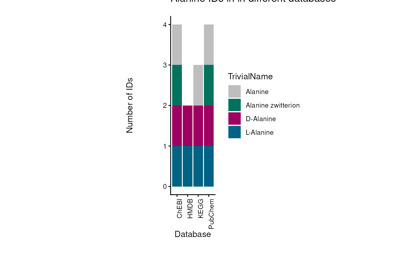
For instance, if we want to assign a HMDB ID, we have to assign both “HMDB0001310” and “HMDB0000161” to the metabolite Alanine. For ChEBI we could assign only one, “16449”, but this may lead to other problems as this ChEBI ID is not specific and may not be part of certain metabolic pathways. The reason for this is that substrate chirality is critical to enzymatic processes, and enzymes are stereoselective, favouring one particular enantiomer (e.g. D-sugars, L-amino acids, etc.).
To showcase the severity of this problem, we can look at the occurrence of those metabolite IDs in metabolic pathways across different databases. To do so, we searched for those metabolite IDs in the RaMP database (Braisted et al. 2023) and extracted the pathways they are part of:

Alanine IDs mapped to pathways from WikiPathways, KEGG and Reactome using RaMP.
TrivialName	ID	Database	PathwayCount
L-Alanine	16977	ChEBI	44
L-Alanine	5950	PubChem	44
L-Alanine	C00041	KEGG	44
L-Alanine	HMDB0000161	HMDB	44
D-Alanine	15570	ChEBI	3
D-Alanine	71080	PubChem	3
D-Alanine	C00133	KEGG	3
D-Alanine	HMDB0001310	HMDB	3
Alanine zwitterion	57383916	PubChem	0
Alanine zwitterion	66916	ChEBI	0
Alanine	16449	ChEBI	4
Alanine	602	PubChem	4
Alanine	C01401	KEGG	4

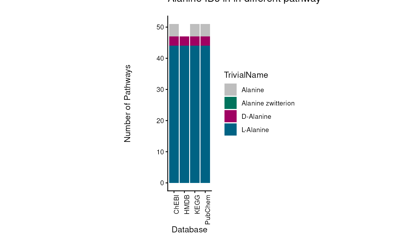
This showcases that if we choose the unspecific ChEBI ID for Alanine (ChEBI ID 16449), because experimentally the distinction was not possible, we will not map to any pathway, even though the metabolite is part of many pathways. Hence, we recommend to assign multiple IDs to a measured peak where specificity in detection is not given.

Yet, many metabolomics studies do not report multiple IDs, but rather one ID per measured peak. In some cases the chosen ID correctly represents the degree of ambiguity in the detection, e.g. “Alanine zwitterion”, whilst in other cases a specific ID is chosen that has not been detected with this specificity, e.g. “L-Alanine”. In both cases this can lead to missed mappings to prior knowledge and hence a loss of information as discussed above.
The function equivalent_id() helps with this: for each measured ID it adds the IDs of equivalent metabolites (e.g. other enantiomers) that may not have been distinguished in the measurement.

# Example Cell-line data:
Input_HMDB <- FeatureMetadata_Cells %>%
    dplyr::filter(!HMDB == "NA") %>% # ID in the measured data we want to use, hence we remove NA's
    dplyr::select("HMDB", "Pathway") # only keep relevant columns

# Add equivalent IDs:
FeatureMetadata_Cells_AddIDs <- equivalent_id(
    data = Input_HMDB,
    metadata_info = c(InputID = "HMDB"), # ID in the measured data, here we use the HMDB ID
    from = "hmdb"
)
#> Warning in equivalent_id(data = Input_HMDB, metadata_info = c(InputID =
#> "HMDB"), : The following IDs are duplicated and removed: HMDB0000725,
#> HMDB0002013, HMDB0000267, HMDB0000755
#> chebi is used to find additional potential IDs for hmdb.

Preview of the DF `FeatureMetadata_Cells_AddIDs` including new columns with potential additional HMDB IDs assigned using the equivalent_id() function.
HMDB	Pathway	PotentialAdditionalIDs
HMDB0000014	Pyrimidine metabolism	NA
HMDB0000033	Not assigned	NA
HMDB0000043	Not assigned	HMDB0059606
HMDB0000045	Purine metabolism	NA
HMDB0000050	Purine metabolism	HMDB0004401, HMDB0004402, HMDB0004421
HMDB0000052	Alanine, aspartate and glutamate metabolism	HMDB0001006
HMDB0000056	Pyrimidine metabolism	NA

The Biocrates kit, which we will use in the rest of this tutorial, has already done this for us: where the measurement is not specific, multiple HMDB IDs are assigned to one feature (e.g. the two HMDB IDs of L- and D-Alanine).

Accessing Prior Knowledge

Metabolite prior knowledge (PK) is essential for the interpretation of metabolomics data. It can be used to perform pathway enrichment analysis and compound class enrichment analysis, and specific PK databases can be used to study the connection of metabolites to receptors or transporters. Since the quality and content of the PK will dictate the success of the downstream analysis and biological interpretation, it is important to ensure the PK is used correctly.
Specifically in metabolite PK, the many different PK databases and resources pose several issues. Indeed, the metabolite identifiers (e.g. KEGG, HMDB, PubChem, etc.) are not standardized across databases, and the same metabolite can have multiple identifiers in different databases. This is known as the many-to-many mapping problem. Moreover, metabolic pathways that are the basis of the PK databases also include co-factors such as ions or other small molecules that are not only part of most reactions, but often cannot be detected in experimentally acquired data (e.g. H2O, CO2, etc).
To address these issues and provide a standardized way to access and integrate metabolite PK, we provide access to several prior knowledge resources from which molecules such as water have been removed. We term this collection of metabolite sets MetSigDB (Metabolite signature database).
In this section we load the resources we need for this tutorial. MetSigDB contains further resources (Reactome, WikiPathways, MACdb), which are introduced and compared in the MetSigDB vignette.

KEGG pathway-metabolite sets

KEGG pathways are loaded via the KEGG API using the package KEGGREST and can be used to perform pathway analysis (Kanehisa and Goto 2000). (KEGG_Pathways)

# This will use KEGGREST to query the KEGG API to load the pathways:
KEGG_Pathways <- metsigdb_kegg()

Preview of the DF `KEGG_Pathways`.
Description	MetaboliteID	term	Metabolite	pubchem	compound_names
map00010	C00022	Glycolysis / Gluconeogenesis	Pyruvate	3324	Pyruvate….
map00010	C00024	Glycolysis / Gluconeogenesis	Acetyl-CoA	3326	Acetyl-C….
map00010	C00031	Glycolysis / Gluconeogenesis	D-Glucose	3333	D-Glucos….
map00030	C00022	Pentose phosphate pathway	Pyruvate	3324	Pyruvate….
map00030	C00031	Pentose phosphate pathway	D-Glucose	3333	D-Glucos….
map00030	C00085	Pentose phosphate pathway	D-Fructose 6-phosphate	3385	D-Fructo….

Chemical class-metabolite sets

The chemical class-metabolite sets are based on the classification of metabolites into chemical classes, which can be used to perform compound class enrichment analysis.
The chemical class-metabolite sets were curated by RaMP-DB, which used ClassyFire (Braisted et al. 2023). Here we access them via OmnipathR.

ChemicalClass_MetabSet <- metsigdb_chemicalclass()
#> Cached file loaded from: ~/.cache/RaMP-ChemicalClass_Metabolite.rds

Preview of the DF `ChemicalClass_MetabSet`.
class_source_id	common_name	ClassyFire_class	ClassyFire_super_class	ClassyFire_sub_class
HMDB0000001	3-Methylhistidine; 1-Methylhistidine	Carboxylic acids and derivatives	Organic acids and derivatives	Amino acids, peptides, and analogues
HMDB0000479	3-Methylhistidine; 1-Methylhistidine	Carboxylic acids and derivatives	Organic acids and derivatives	Amino acids, peptides, and analogues
HMDB0000005	2-Ketobutyric acid	Keto acids and derivatives	Organic acids and derivatives	Short-chain keto acids and derivatives
HMDB0000008	2-Hydroxybutyric acid	Hydroxy acids and derivatives	Organic acids and derivatives	Alpha hydroxy acids and derivatives
HMDB0000010	2-Methoxyestrone	Steroids and steroid derivatives	Lipids and lipid-like molecules	Estrane steroids
HMDB0000172	L-Isoleucine	Carboxylic acids and derivatives	Organic acids and derivatives	Amino acids, peptides, and analogues
HMDB0000174	L-Fucose	Organooxygen compounds	Organic oxygen compounds	Carbohydrates and carbohydrate conjugates
HMDB0000175	Inosinic acid	Purine nucleotides	Nucleosides, nucleotides, and analogues	Purine ribonucleotides
HMDB0000176	Maleic acid	Carboxylic acids and derivatives	Organic acids and derivatives	Dicarboxylic acids and derivatives
HMDB0000783	Propionylglycine	Carboxylic acids and derivatives	Organic acids and derivatives	Amino acids, peptides, and analogues
HMDB0000784	Azelaic acid	Fatty Acyls	Lipids and lipid-like molecules	Fatty acids and conjugates
HMDB0000785	N-Acetyl-7-O-acetylneuraminic acid	Organooxygen compounds	Organic oxygen compounds	Carbohydrates and carbohydrate conjugates
HMDB0000786	Alloxan; Oxypurinol	Imidazopyrimidines	Organoheterocyclic compounds	Purines and purine derivatives

Create pathway-metabolite sets

The function make_gene_metab_set() can be used to convert gene names to metabolite names by using a PK network of metabolic reactions called CosmosR (Dugourd et al. 2021). This function is useful if you want to perform pathway enrichment analysis on available gene-sets such as the Hallmarks gene-sets from MSigDB (Castanza et al. 2022). Moreover, it enables you to perform combined pathway enrichment analysis on metabolite-gene sets, if you have other data types such as proteomics measuring the enzyme expression.
The Hallmarks (Liberzon et al. 2015) gene-sets and the Gaude (Gaude and Frezza 2016) gene-sets are available in the package MetaProViz and can be loaded using data(hallmarks) and data(gaude_pathways) respectively.

# Load the example gene-sets:
data(hallmarks)
Hallmark_Pathways <- hallmarks

data(gaude_pathways)
Gaude_Pathways <- gaude_pathways

Preview of the DF `Hallmark_Pathways` including gene-sets usable for pathway enrichment analysis.
term	gene
HALLMARK_BILE_ACID_METABOLISM	GSTK1
HALLMARK_BILE_ACID_METABOLISM	ABCG4
HALLMARK_GLYCOLYSIS	LDHC
HALLMARK_GLYCOLYSIS	ARPP19
HALLMARK_GLYCOLYSIS	LDHC
HALLMARK_GLYCOLYSIS	ARPP19
HALLMARK_GLYCOLYSIS	CENPA

Preview of the DF `Gaude_Pathways` including gene-sets usable for pathway enrichment analysis.
gene	term	UniqueGene
CPT1A	Carnitine shuttle	Unique
CPT1B	Carnitine shuttle	Unique
CPT1C	Carnitine shuttle	Unique
CPT2	Carnitine shuttle	Unique
CRAT	Carnitine shuttle	Unique
SLC22A4	Carnitine shuttle	In multiple Pathways
SLC22A5	Carnitine shuttle	In multiple Pathways
SLC25A20	Carnitine shuttle	In multiple Pathways
ACO1	Citric Acid Cycle	Unique
ACO2	Citric Acid Cycle	Unique
GOT1	Citric Acid Cycle	In multiple Pathways

Now we can use the function make_gene_metab_set() to translate the gene names to metabolite names.

# Translate gene names to metabolite names
Hallmarks_GeneMetab <- make_gene_metab_set(
    input_pk = Hallmark_Pathways,
    metadata_info = c(Target = "gene"),
    pk_name = "Hallmarks"
)

Gaude_GeneMetab <- make_gene_metab_set(
    input_pk = Gaude_Pathways,
    metadata_info = c(Target = "gene"),
    pk_name = "Gaude"
)

Preview of the DF `Hallmarks_GeneMetab` including gene-metabolite-sets usable for pathway enrichment analysis.
term	feature
HALLMARK_GLYCOLYSIS	ME2
HALLMARK_GLYCOLYSIS	LDHC
HALLMARK_GLYCOLYSIS	FKBP4
HALLMARK_GLYCOLYSIS	HMDB0000241
HALLMARK_GLYCOLYSIS	HMDB0000570
HALLMARK_GLYCOLYSIS	HMDB0000122

Given that we have the gene-metabolite-sets, we can now also run enrichment analysis on combined data types, including both the metabolite Log2FC and the gene Log2FC from e.g. transcriptomics or proteomics data. Yet, it is important to keep in mind that generally we detect fewer metabolites than genes and hence this may bias the results obtained from combined enrichment analysis.

MetaLinksDB metabolite-receptor & metabolite-transporter sets

The MetaLinks database is a manually curated database of metabolite-receptor and metabolite-transporter sets that can be used to study the connection of metabolites and receptors or transporters (Farr et al. 2024).

MetaLinksDB <- metsigdb_metalinks()

Preview of the DF `MetaLinksDB` including metabolite-receptor sets.
metabolite	protein_name	type	mor	transport_direction	combined_score	mode_of_regulation	protein_type_clean	receptor_class
Pentadecanal	NA	Production-Degradation	1	NA	NA	Activating	NA	NA
Adenosine triphosphate	NA	Production-Degradation	-1	NA	NA	Inhibiting	NA	NA
3-Oxooctadecanoyl-CoA	NA	Production-Degradation	1	NA	NA	Activating	NA	NA
Malonyl-CoA	NA	Production-Degradation	-1	NA	NA	Inhibiting	NA	NA
Triiodothyronine sulfate	NA	Production-Degradation	1	NA	NA	Activating	NA	NA
Adenosine monophosphate	NA	Production-Degradation	-1	NA	NA	Inhibiting	NA	NA

Preview of the metabolite-receptor and metabolite-transporter sets.
metabolite	protein_name	gene_symbol	uniprot	hmdb	type	mor	transport_direction	protein_type	source	experiment_score	combined_score	mode_of_regulation	protein_type_clean	receptor_class	interaction_family	interaction_annotation_status	interaction_mechanism	regulation_polarity	transport_direction_label	transport_mode	evidence_class	experiment_evidence_present	combined_confidence_tier	interaction_detail	interaction	direction	term_specific
D-Fructose	NA	SLC5A10	A0PJK1	HMDB0000660	Production-Degradation	1	out	“transporter”	recon	NA	NA	Activating	transporter	NA	Transporter-metabolite	transporter_with_pd_edge	Transport	Positive (activating)	Export/Secretion	Efflux transporter	Metabolic knowledgebase	No/Unknown	Unknown	Efflux transporter; Positive (activating)	Transport_Out	to_term	transporter_Production-Degradation
Heneicosanoic acid	NA	FABP12	A6NFH5	HMDB0002345	Production-Degradation	1	out	“other_protein”	recon	NA	NA	Activating	other_protein	NA	Transporter-metabolite	transporter_with_pd_edge	Transport	Positive (activating)	Export/Secretion	Efflux transporter	Metabolic knowledgebase	No/Unknown	Unknown	Efflux transporter; Positive (activating)	Transport_Out	to_term	other_protein_Production-Degradation
L-Glutamic acid	NA	GRM8	O00222	HMDB0000148	Ligand-Receptor	1	NA	“gpcr”	CellPhoneDB	0	986	Activating	gpcr	GPCR	Receptor-metabolite	source_annotations_concordant_or_incomplete	Ligand-receptor signaling	Positive (activating)	Not specified	NA	Cell-cell communication resource	No/Unknown	Very high	GPCR; Positive (activating)	Ligand-Receptor	to_term	gpcr_Ligand-Receptor
12-HETE	NA	GPR31	O00270	HMDB0006111	Ligand-Receptor	0	NA	“gpcr”	Stitch	0	907	Binding	gpcr	GPCR	Receptor-metabolite	source_annotations_concordant_or_incomplete	Ligand-receptor signaling	Neutral (binding)	Not specified	NA	Chemical-protein interaction resource	No/Unknown	Very high	GPCR; Neutral (binding)	Ligand-Receptor	to_term	gpcr_Ligand-Receptor

Comparison of PK coverage

We have now loaded a number of different PK sources (details above) and aim to compare the overlap in coverage between these PK sources to understand if there are certain genes or metabolites covered by one PK resource but not the others. As an example, we will compare the resources containing gene-metabolite sets (Hallmarks, Gaude, MetaLinksDB) using the compare_pk() function, which generates a combined data table and visualises it as an upset plot. The upset plot shows the overlap of coverage, similar to how a Venn diagram works, but enables us to visualise many combinations clearly.

# Compare the PK resources
pk_comp_res <- compare_pk(
    data = list(
        Hallmarks = as.data.frame(Hallmarks_GeneMetab[["GeneMetabSet"]]),
        Gaude = as.data.frame(Gaude_GeneMetab[["GeneMetabSet"]]),
        MetalinksDB = as.data.frame(MetaLinksDB)
    )
)
#> Warning: `aes_string()` was deprecated in ggplot2 3.0.0.
#> ℹ Please use tidy evaluation idioms with `aes()`.
#> ℹ See also `vignette("ggplot2-in-packages")` for more information.
#> ℹ The deprecated feature was likely used in the MetaProViz package.
#>   Please report the issue at <https://github.com/saezlab/MetaProViz/issues>.
#> This warning is displayed once per session.
#> Call `lifecycle::last_lifecycle_warnings()` to see where this warning was
#> generated.
#> Warning: Using `size` aesthetic for lines was deprecated in ggplot2 3.4.0.
#> ℹ Please use `linewidth` instead.
#> ℹ The deprecated feature was likely used in the ComplexUpset package.
#>   Please report the issue at
#>   <https://github.com/krassowski/complex-upset/issues>.
#> This warning is displayed once per session.
#> Call `lifecycle::last_lifecycle_warnings()` to see where this warning was
#> generated.

The table includes all features of the three PK resources we decided to compare. Additionally, it includes a column for each PK resource with value 1 if the feature is present in the PK resource and 0 if it is not. The column “Type” specifies which ID type the feature corresponds to, here either metabolite (HMDB) or gene, which is used for visualisation purposes in the upset plot.

Preview of the DF `pk_comp_res$summary_table` showing coverage of features (genes or metabolites) across PK sources.
Feature	Hallmarks	Gaude	MetalinksDB	Type
FABP4	1	0	1	gene
ADIPOQ	1	0	0	gene
PPARG	1	0	1	gene
LIPE	1	0	1	gene
DGAT1	1	1	1	gene
LPL	1	1	1	gene
CPT2	1	1	1	gene
CD36	1	0	1	gene

The upset plot shows that MetaLinksDB has unique genes and metabolites not present in the other resources. This is to be expected, since MetaLinksDB focuses on receptors, transporters and metabolic enzymes, whilst Gaude and Hallmarks focus on pathways.
Since Gaude only focuses on metabolic enzymes of pathways, it contains a low number of genes and hence has a small amount of unique genes and metabolites. In this regard it makes sense that Hallmarks includes many unique genes, since Hallmarks also includes other genes and pathways not related to metabolism. Between Hallmarks and Gaude we observe a high overlap of metabolites. This can be explained since both gene-sets are assigned metabolites by using the same metabolic reaction network in the backend of make_gene_metab_set(), and it is important to keep in mind that this network dictates the gene-metabolite associations added.

Linking experimental data to prior knowledge

Now that we have loaded the prior knowledge and inspected the overlap of genes and metabolites between the different PK resources, in this section we want to link our experimental data to the PK.
Whichever resource the experimental data resembles, we recommend to follow this overall approach:

1. Determine the metabolite identifiers from the experimental data and inspect their coverage.
2. Select the metabolite identifiers from the experimental data, which can be used to link to the PK of interest.
3. Connect the metabolite identifiers to the PK and assess the overlap.

Here one can select any combination of experimental data and PK. This selection should be based on the experimental data at hand and the biological research question.
For this tutorial, we will focus on the combination of the Biocrates experimental data and the MetaLinksDB PK. The reason for using the landscape of metabolites included in the Biocrates kit is that Biocrates has assigned multiple types of metabolite IDs to each measurement (LIPID MAPS, HMDB, ChEBI) and, where needed, multiple IDs of one type to one measurement (e.g. the two HMDB IDs of L- and D-Alanine).

Determine identifiers and inspect coverage

First we determine the identifiers and inspect the coverage.
In experimentally acquired data, different metabolite IDs can be used to describe a metabolite. In the Biocrates data the available metabolite identifiers that could be linked to PK resources are mostly ChEBI, HMDB, and LIPID MAPS (LIMID). We now select these metabolite identifier columns to count the coverage and look at the combinations of the coverage grouped by the class of metabolite. This helps us to understand what to expect when linking the data to prior knowledge.

pk_comp_res_biocft <- compare_pk(
    data = list(Biocft = FeatureMetadata_Biocrates),
    metadata_info = list(Biocft = c("CHEBI", "HMDB", "LIMID")),
    plot_name = "Overlap of BioCrates Columns",
    print_plot = FALSE
)

Preview of the DF `pk_comp_res_biocft$summary_table` showing coverage of identifiers.
TrivialName	CHEBI	HMDB	LIMID	Class
1-Met-His	1	1	0	Aminoacids Related
3-IAA	1	1	0	Indoles Derivatives
3-IPA	1	1	0	Indoles Derivatives
3-Met-His	1	1	0	Aminoacids Related
5-AVA	1	1	1	Aminoacids Related
AABA	1	1	1	Aminoacids Related
AbsAcid	1	1	1	Hormones
Ac-Orn	1	1	0	Aminoacids Related

These results tell us that:

Less than half of the metabolites have CHEBI+HMDB+LIMID (n=413), which isn’t great, but probably higher than we would have expected.
If you relied only upon:
- CHEBI: then you would miss at least 256 metabolites with HMDB+LIMID
- HMDB: then you would miss at least 54 metabolites with CHEBI+LIMID
- LIMID: then you would miss at least 89 metabolites with CHEBI+HMDB

However, there are two things to note about these observations.

The first is that these numbers are minimums; the real values are a little higher once you add, for instance, metabolites with just CHEBI or just LIMID. So actually, relying upon only LIMID means we miss 151 Biocrates metabolites (89 with only HMDB/ChEBI + 15 with only CHEBI + 8 with only HMDB and 39 with no LIMID/CHEBI/HMDB identifiers).

The second point is more nuanced but just as important: there is no direct 1:1 relationship between the number of Biocrates metabolites with, for instance, a ChEBI ID, and the number of unique ChEBI IDs that they map to. The upset plot treats each Biocrates metabolite as an individual entry and categorises whether it has a ChEBI, HMDB, LIMID ID, etc. However, it does not consider what those ChEBI, HMDB or LIMID IDs actually are. So it is possible that the number of metabolites is higher, or lower, than the number of unique IDs due to multi-mapping.

For example, assume we have 3 Biocrates metabolites with only HMDB IDs. These count as 3 entries in the upset plot. But two of these Biocrates metabolites could both map to the same HMDB ID, whereas the third Biocrates metabolite could map to 6 different HMDB IDs. In this case, there are 3 Biocrates metabolites with HMDB IDs but 7 unique HMDB IDs. Hence, it is important to keep this in mind when interpreting the upset plot.

Select identifiers to link to PK of interest

We have inspected the experimental coverage of the metabolite IDs from the Biocrates kit. Next, we have to choose which metabolite identifier to use to link to the PK of choice. Often this choice is dictated by the prior knowledge resource, as most of them use a specific identifier.
Here we will use MetaLinksDB, which uses HMDB IDs as metabolite identifiers, hence it is best to use the HMDB IDs to link the Biocrates features to the resource. Noteworthy, in some cases the Biocrates metabolites have multiple HMDB IDs listed per metabolite. We can count them using count_id():

# Count entries and record NA information
result_bioc_hmdb_count <- count_id(FeatureMetadata_Biocrates, "HMDB", delimiter = ", ")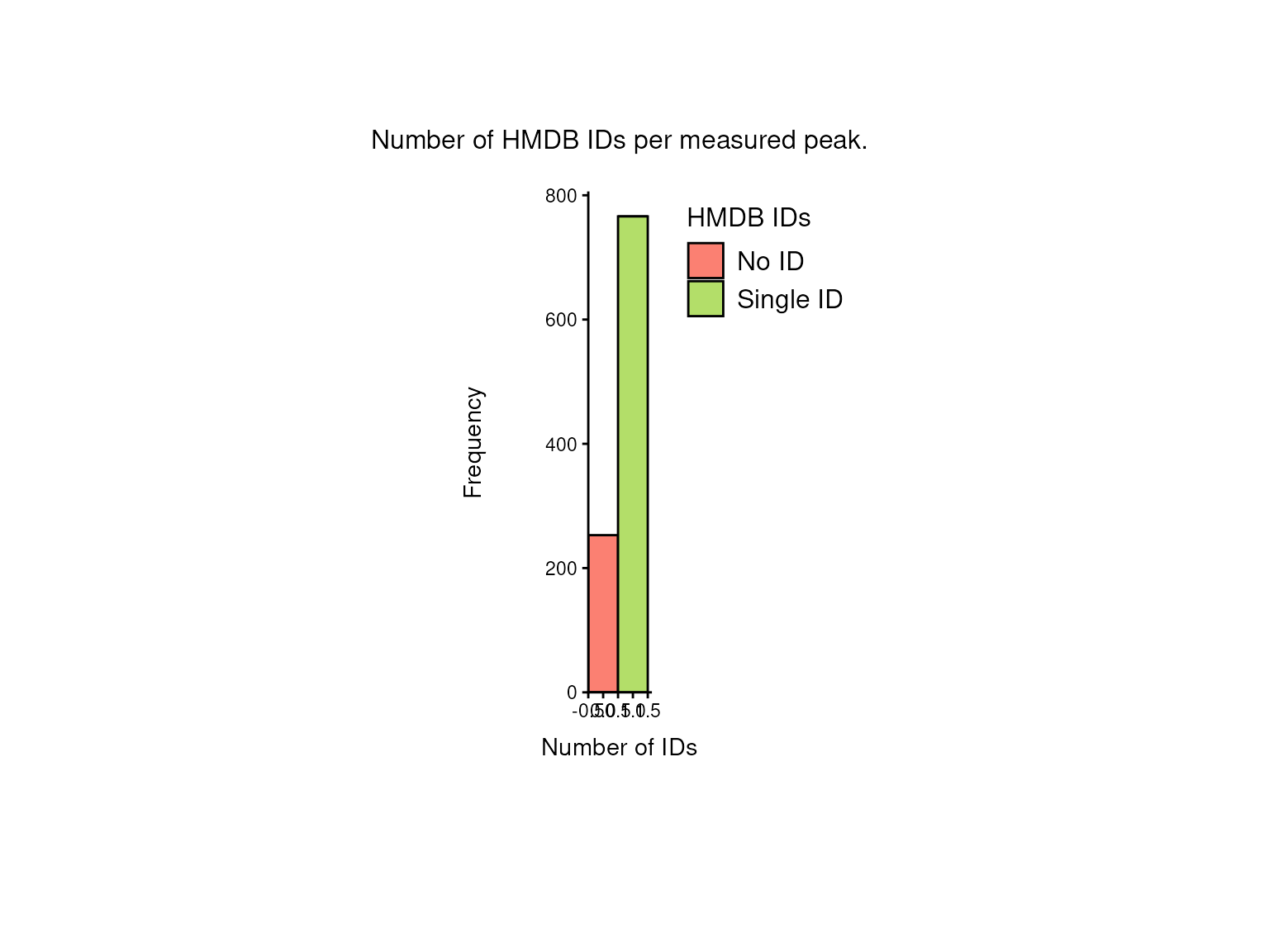

# Access the processed data:
processed_df_bioc_hmdb_count <- result_bioc_hmdb_count$Table

From this plot we can make a few observations:
1. The number of Biocrates features without any HMDB ID is very high (n=253).
2. Whilst a number of Biocrates features have only a single HMDB ID associated with them (n=314), the majority of Biocrates metabolites actually have multiple entries (n=452).
3. For those with multiple, this ranges from 2-20 HMDB IDs per Biocrates feature!

With so many Biocrates features linked to multiple HMDB IDs there are different ways to deal with this (e.g. select a single HMDB ID in cases where we have multiple). We discuss the pros and cons of this in section 3.4 Are multiple metabolite IDs helpful or a hindrance?. For now, we proceed with making the connections to the PK using all HMDB IDs, which the MetaProViz function checkmatch_pk_to_data() has been designed to handle.

Make connection to PK and assess overlap

Here we connect the experimental Biocrates table to the MetaLinksDB PK via the HMDB IDs using the checkmatch_pk_to_data() function.

Biocrates_to_MetalinksDB <- checkmatch_pk_to_data(
    data = FeatureMetadata_Biocrates,
    input_pk = MetaLinksDB,
    metadata_info = c(InputID = "HMDB", PriorID = "hmdb", grouping_variable = NULL)
)
#> Warning in checkmatch_pk_to_data(data = FeatureMetadata_Biocrates, input_pk =
#> MetaLinksDB, : 253 NA values were removed from column HMDB
#> Warning in checkmatch_pk_to_data(data = FeatureMetadata_Biocrates, input_pk =
#> MetaLinksDB, : 4 duplicated IDs were removed from column HMDB
#> No metadata_info grouping_variable provided. If this was not intentional, please check your input.
#> Warning in checkmatch_pk_to_data(data = FeatureMetadata_Biocrates, input_pk =
#> MetaLinksDB, : 35390 duplicated IDs were removed from PK column hmdb
#> data has multiple IDs per measurement = TRUE. input_pk has multiple IDs per entry = FALSE.
#> data has 762 unique entries with 2027 unique HMDB IDs. Of those IDs, 176 match, which is 8.68278243709916%.
#> input_pk has 1116 unique entries with 1116 unique hmdb IDs. Of those IDs, 176 are detected in the data, which is 15.7706093189964%.
#> Warning in checkmatch_pk_to_data(data = FeatureMetadata_Biocrates, input_pk =
#> MetaLinksDB, : There are cases where multiple detected IDs match to multiple
#> prior knowledge IDs of the same category

This returns some warning messages and three tables:

data_summary: a summary table with the links to the prior knowledge, including pointers if any action is required. Any NA values or duplicates of the InputID (e.g. ‘HMDB’) are removed from this table.
GroupingVariable_summary: an extended version of the summary, where the grouping variable is taken into account, e.g. for pathway-metabolite sets this would include duplicated InputIDs as they are in multiple pathways.
data_long: an all-versus-all comparison to enable checking on a case-by-case basis.

In some cases we expect only one input ID to be linked to one entry in the PK. But this won’t always be the case, and as already discussed in the last section, in many cases here we have multiple HMDB IDs per single Biocrates feature. checkmatch_pk_to_data() has been designed with this in mind: by default it splits any comma separated values in the InputID (or PriorID) into separate entities, counts the number of links between these, and reports this to the user.

Let’s take a look at the results:

Preview of the DF `data_summary` showing coverage of identifiers (some columns hidden)
HMDB	matches	original_count	matches_count	GroupingVariable	Count_FeatureIDs_to_GroupingVariable	Group_Conflict_Notes	Unique_GroupingVariable_count	ActionRequired	InputID_select	Action_Specific
HMDB0000001	NA	1	0	NA	NA	None	0	None	HMDB0000001	None
HMDB0000033	NA	1	0	NA	NA	None	0	None	HMDB0000033	None
HMDB0000036	HMDB0000036	1	1	OneGroup	1	None	1	None	HMDB0000036	None
HMDB0000043	HMDB0000043	1	1	OneGroup	1	None	1	None	HMDB0000043	None
HMDB0000056	HMDB0000056	1	1	OneGroup	1	None	1	None	HMDB0000056	None
HMDB0000062	HMDB0000062	1	1	OneGroup	1	None	1	None	HMDB0000062	None
HMDB0000063	HMDB0000063	1	1	OneGroup	1	None	1	None	HMDB0000063	None
HMDB0000072, HMDB0000958	NA	2	0	NA, NA	NA, NA	None	0	None	HMDB0000072	None

For a few metabolite classes of the Biocrates kit, every metabolite has a HMDB ID and a corresponding entry in MetaLinksDB. For a number of other classes, however, we see that they are not represented in the MetaLinksDB PK at all, either because there is no HMDB ID associated with the Biocrates metabolite, or because MetaLinksDB does not include the HMDB ID of that metabolite.
This poor coverage could be a concern if we are interested in analysing many of these classes, since it means that our experimental results for e.g. Phosphatidylglycerols will not be linked to PK. In any case we need to keep this in mind for downstream analysis and the interpretation of results, so that we don’t overinterpret results that, for instance, include a large number of amino acids, or falsely assume that the absence of Phosphatidylinositols in our PK integration results means that they are not present or important in our data.

Are multiple metabolite IDs helpful or a hindrance?

Let’s turn back to the number of HMDB IDs we have in the Biocrates data and ask ourselves: is it helpful or detrimental to have multiple IDs? To answer this, we take only the first HMDB ID of each feature with multiple HMDB IDs, repeat the matching and compare the number of matches.

# Number of matches using all HMDB IDs:
MultipleIDs <- Biocrates_to_MetalinksDB$data_summary %>%
    summarise(total_matches_count = sum(matches_count, na.rm = TRUE)) %>%
    mutate(Name = "MultipleIDs")

# Extract first ID:
extract_first_id <- function(id_col) {
    map_chr(as.character(id_col), function(x) {
        # Check for NA or empty string
        if (is.na(x) || x == "") {
            return(NA)
        }
        # Split on comma (adjust the delimiter if needed)
        parts <- unlist(strsplit(x, split = ","))
        # Return the first value after trimming any whitespace
        return(trimws(parts[1]))
    })
}

# Create a copy of the df
FeatureMetadata_Biocrates_singleHMDB <- FeatureMetadata_Biocrates
# Get the first entry of each HMDB ID
FeatureMetadata_Biocrates_singleHMDB$HMDB_single <- extract_first_id(FeatureMetadata_Biocrates$HMDB)

# Visually check that the single ID function has worked:
result_bioc_hmdb_count_single <- count_id(FeatureMetadata_Biocrates_singleHMDB, "HMDB_single")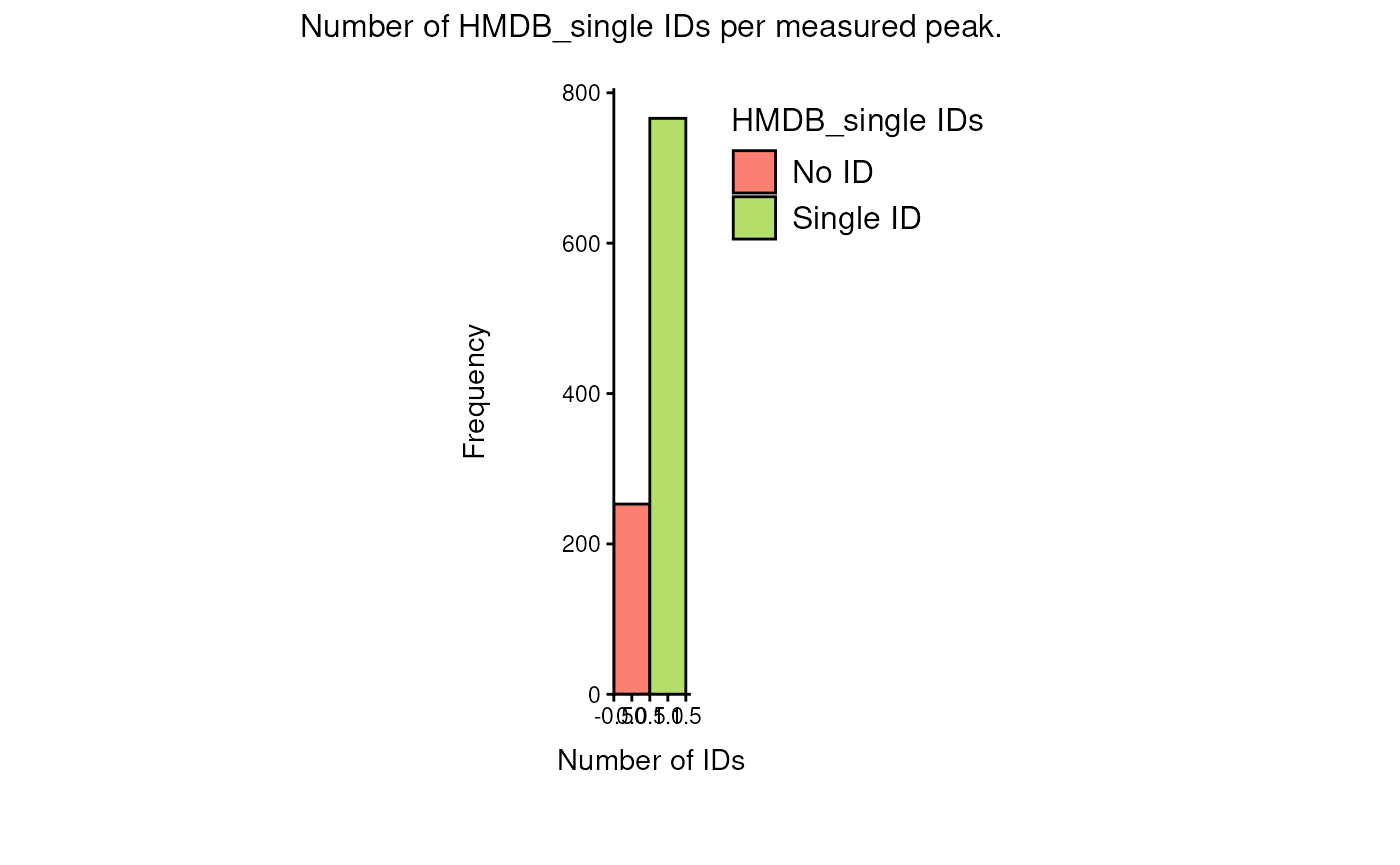


# Check the matches:
Biocrates_to_MetalinksDB_singleHMDB <- checkmatch_pk_to_data(
    data = FeatureMetadata_Biocrates_singleHMDB,
    input_pk = MetaLinksDB,
    metadata_info = c(InputID = "HMDB_single", PriorID = "hmdb", grouping_variable = NULL)
)
#> Warning in checkmatch_pk_to_data(data = FeatureMetadata_Biocrates_singleHMDB, :
#> 253 NA values were removed from column HMDB_single
#> Warning in checkmatch_pk_to_data(data = FeatureMetadata_Biocrates_singleHMDB, :
#> 49 duplicated IDs were removed from column HMDB_single
#> No metadata_info grouping_variable provided. If this was not intentional, please check your input.
#> Warning in checkmatch_pk_to_data(data = FeatureMetadata_Biocrates_singleHMDB, :
#> 35390 duplicated IDs were removed from PK column hmdb
#> data has multiple IDs per measurement = FALSE. input_pk has multiple IDs per entry = FALSE.
#> data has 717 unique entries with 717 unique HMDB_single IDs. Of those IDs, 147 match, which is 20.5020920502092%.
#> input_pk has 1116 unique entries with 1116 unique hmdb IDs. Of those IDs, 147 are detected in the data, which is 13.1720430107527%.

# Number of matches using a single HMDB ID:
SingleIDs <- Biocrates_to_MetalinksDB_singleHMDB$data_summary %>%
    summarise(total_matches_count = sum(matches_count, na.rm = TRUE)) %>%
    mutate(Name = "SingleID")

# Compare:
bind_rows(MultipleIDs, SingleIDs) %>%
    preview_table(caption = "Comparison of IDs found in the MetaLinksDB PK when having multiple versus a single HMDB ID in the measured data.", row.names = FALSE)

Comparison of IDs found in the MetaLinksDB PK when having multiple versus a single HMDB ID in the measured data.
total_matches_count	Name
208	MultipleIDs
147	SingleID

This shows that using multiple HMDB IDs has resulted in more metabolites from Biocrates being linked to MetaLinksDB than would have been possible if we only used the first HMDB ID available to us. Hence, while having multiple IDs for a single detected peak may add complexity, we recommend against prematurely dropping any IDs until you have mapped to the PK or have thoroughly assessed what impact the removal may have.

Deeper investigation of MetaLinksDB metabolite-protein interactions

Now that we have investigated the coverage of metabolite ID annotations and their matches to prior knowledge, we can go a step further and look into the interactions of the measured metabolites with transporters, receptors and metabolic enzymes. For that, we subset MetaLinksDB by the “interaction_family” column, which contains one of the following categories: “Other protein-metabolite”, “Transporter-metabolite”, “Receptor-metabolite”, and “Enzyme-metabolite”, and visualise each subset using the viz_pk_network() function.

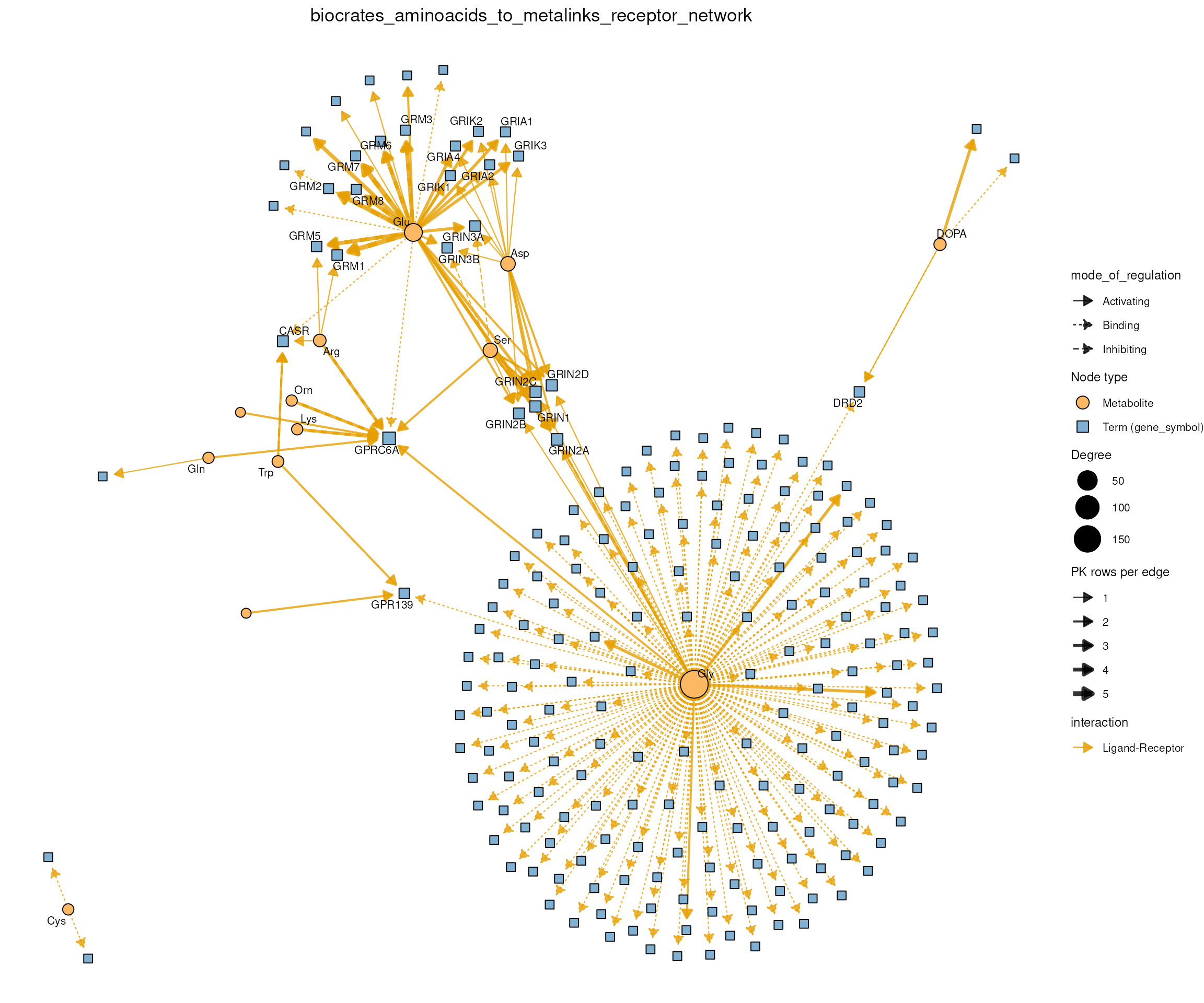
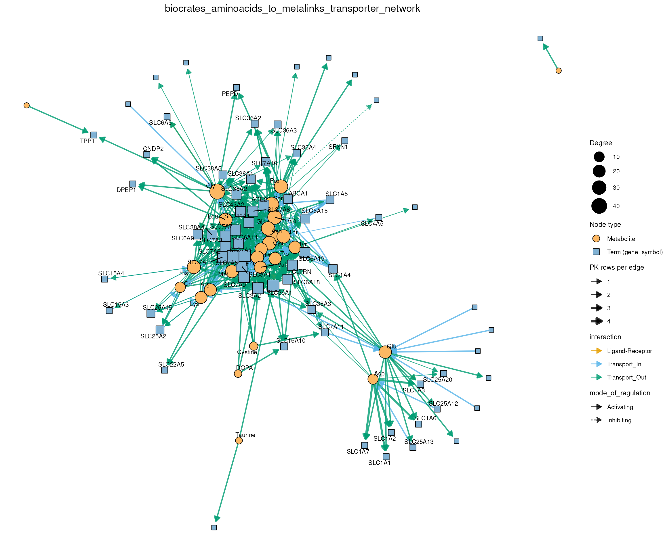
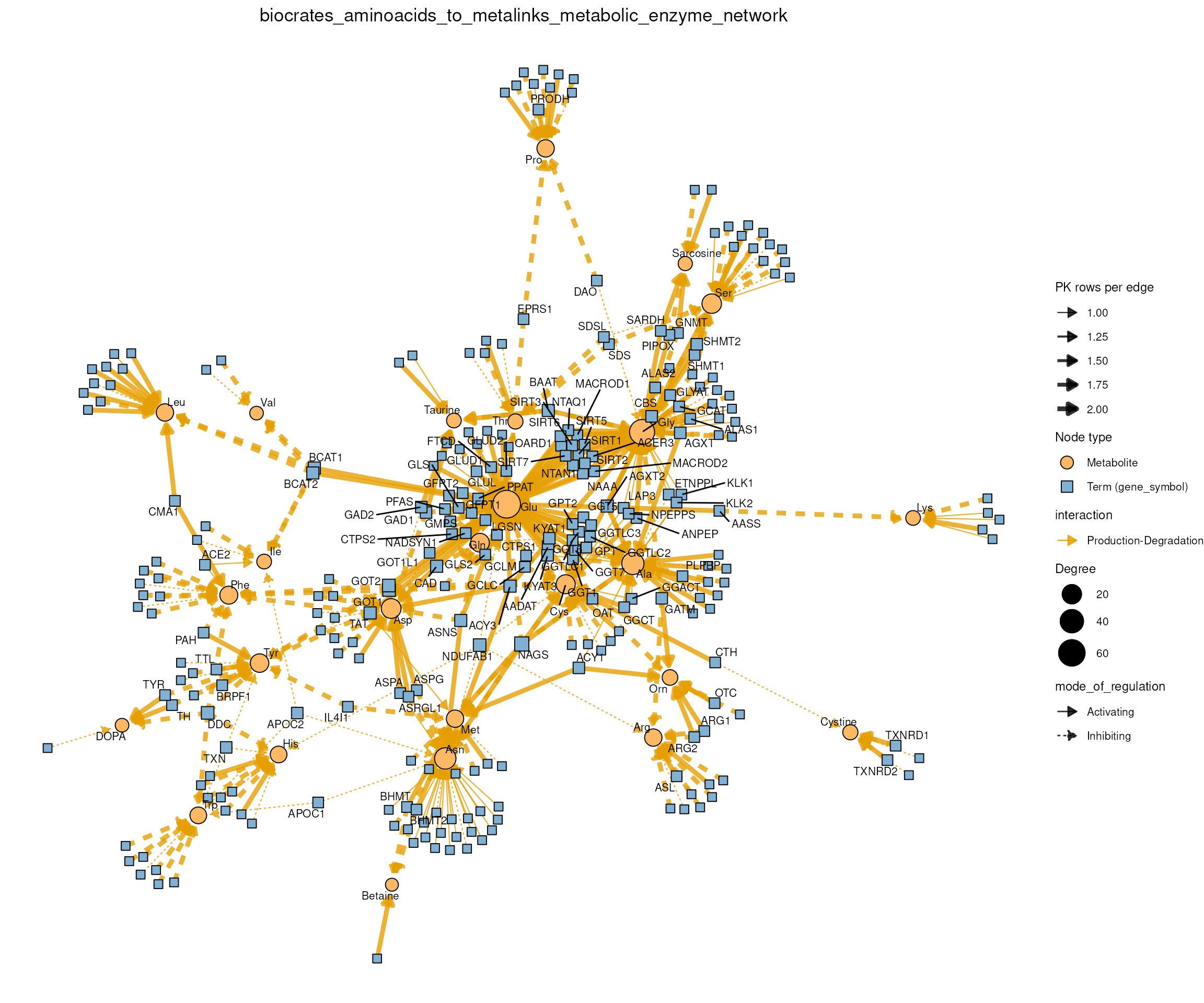
Due to the number of Biocrates features and the size of MetaLinksDB, these visualisations quickly become convoluted. Hence, we only investigate the amino acid subset of the Biocrates features.

# Get MetaLinksDB subsets based on interaction_family:
metalinks_receptor <- MetaLinksDB %>% filter(interaction_family == "Receptor-metabolite")
metalinks_transporter <- MetaLinksDB %>% filter(interaction_family == "Transporter-metabolite")
metalinks_metabolic_enzyme <- MetaLinksDB %>% filter(interaction_family == "Enzyme-metabolite")

# Subset biocrates_features to amino acids:
biocrates_amino_acids <- biocrates_features %>%
    filter(
        Class %in% c("Aminoacids Related", "Aminoacids")
    )

# Columns to match the Biocrates features to MetaLinksDB and to style the network:
metalinks_info <- c(
    InputID = "HMDB",
    InputLabel = "TrivialName",
    PriorID = "hmdb",
    PriorTerm = "gene_symbol",
    EdgeColor = "interaction",
    EdgeLinetype = "mode_of_regulation",
    EdgeDirection = "direction"
)

Plot the metabolite-protein interaction network of the Biocrates amino acids and MetaLinksDB receptors:

# receptor-network
biocrates_metalinks_receptor <- viz_pk_network(
    feature_metadata = biocrates_amino_acids,
    input_pk = metalinks_receptor,
    metadata_info = metalinks_info,
    id_sep = ",",  # biocrates_features has possibly multiple HMDB IDs per feature, separated by ", "
    label_mode = "reduced",
    plot_name = "biocrates_aminoacids_to_metalinks_receptor_network",
    save_plot = NULL
)

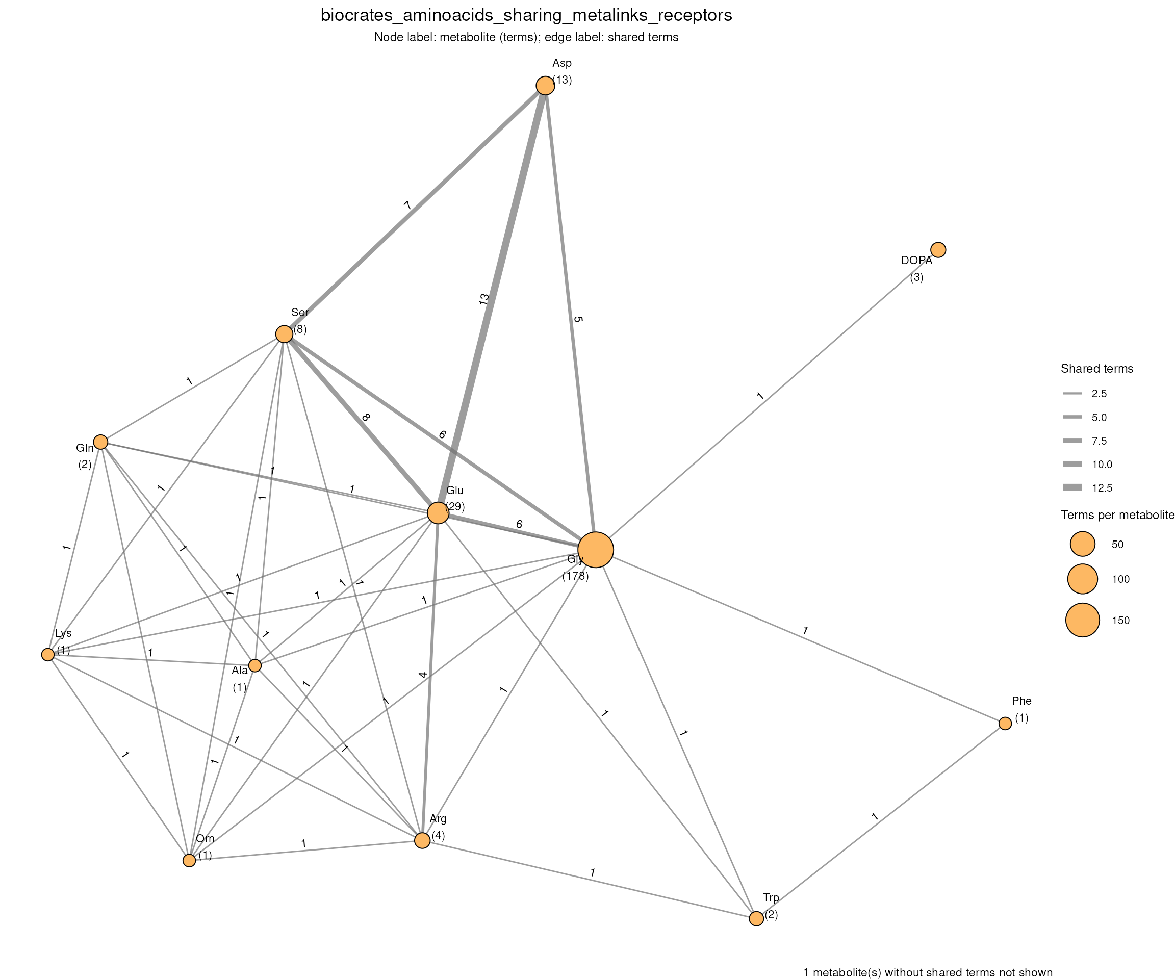
While the network above shows the specific interactions of metabolites with proteins, viz_shared_pk_network() shows how the metabolites share interactions with the same proteins. It takes the same inputs:

# receptor-sharing
biocrates_metalinks_receptor_shared <- viz_shared_pk_network(
    feature_metadata = biocrates_amino_acids,
    input_pk = metalinks_receptor,
    metadata_info = metalinks_info,
    id_sep = ",",
    plot_name = "biocrates_aminoacids_sharing_metalinks_receptors",
    save_plot = NULL
)

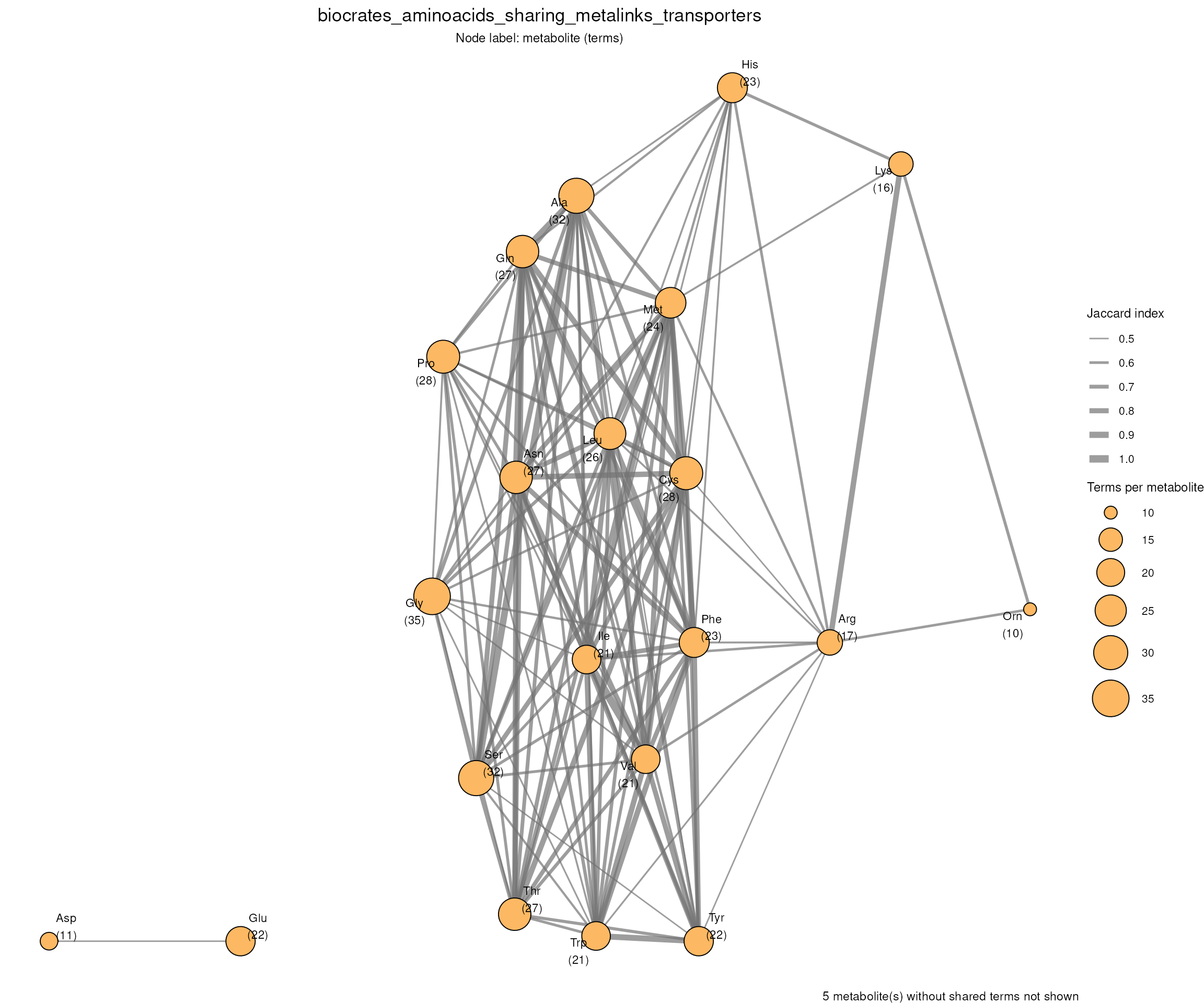
Plot the metabolite-protein interaction network of the Biocrates amino acids and MetaLinksDB transporters, and how the amino acids share transporters:

# transporter-network
biocrates_metalinks_transporter <- viz_pk_network(
    feature_metadata = biocrates_amino_acids,
    input_pk = metalinks_transporter,
    metadata_info = metalinks_info,
    id_sep = ",",
    label_mode = "reduced",
    plot_name = "biocrates_aminoacids_to_metalinks_transporter_network",
    save_plot = NULL
)


# Most amino acids share some transporters. To focus on the strongly
# overlapping pairs we use the Jaccard index with a threshold and omit
# the edge labels, as the edge width shows the Jaccard index as well:
biocrates_metalinks_transporter_shared <- viz_shared_pk_network(
    feature_metadata = biocrates_amino_acids,
    input_pk = metalinks_transporter,
    metadata_info = metalinks_info,
    similarity = "jaccard",
    threshold = 0.5,
    edge_labels = FALSE,
    id_sep = ",",
    plot_name = "biocrates_aminoacids_sharing_metalinks_transporters",
    save_plot = NULL
)

Plot the metabolite-protein interaction network of the Biocrates amino acids and MetaLinksDB metabolic enzymes, and how the amino acids share metabolic enzymes:

# metabolic-enzyme-network
biocrates_metalinks_metabolic_enzyme <- viz_pk_network(
    feature_metadata = biocrates_amino_acids,
    input_pk = metalinks_metabolic_enzyme,
    metadata_info = metalinks_info,
    id_sep = ",",
    label_mode = "reduced",
    plot_name = "biocrates_aminoacids_to_metalinks_metabolic_enzyme_network",
    save_plot = NULL
)


biocrates_metalinks_metabolic_enzyme_shared <- viz_shared_pk_network(
    feature_metadata = biocrates_amino_acids,
    input_pk = metalinks_metabolic_enzyme,
    metadata_info = metalinks_info,
    id_sep = ",",
    plot_name = "biocrates_aminoacids_sharing_metalinks_metabolic_enzymes",
    save_plot = NULL
)

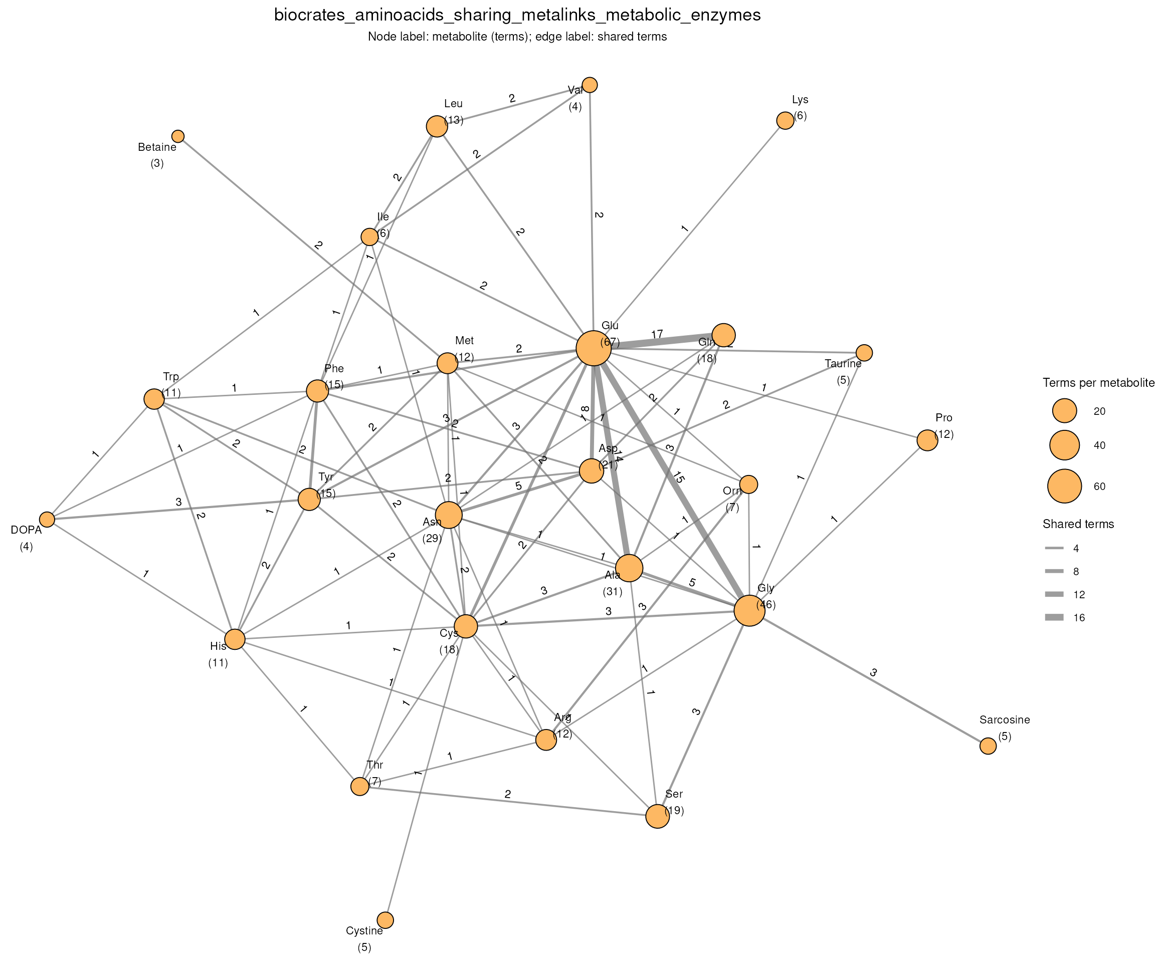
In the sharing networks, the number beneath each metabolite is its total number of interacting proteins and the edge labels show the number of shared proteins. For example, in the receptor subset of MetaLinksDB, we observe many interactions for Glutamic acid (Glu) and Glycine (Gly). Indeed, the corresponding sharing plot shows that Gly and Glu share 6 proteins which they interact with. Additionally, we see that Glu and Asp (Aspartic acid) share 13 receptors, which are all 13 receptors of Asp, while Glu interacts with 29 receptors, hinting at a possibly higher receptor specificity of Aspartic acid in comparison to a more versatile interaction profile of Glutamic acid. As the raw number of shared proteins favours metabolites with many interactions, viz_shared_pk_network() can also use the Jaccard index (Jaccard 1901) as edge weight (parameter similarity), as we did for the transporters above. More examples are shown in the CoRe Metabolomics vignette. Note, however, that metabolite-protein interactions have various interaction properties and binding mechanisms, and that prior knowledge resources are always biased towards well-studied small molecules and proteins. Therefore, the overlap graph hints at shared protein interactions, but does not show that two metabolites interact with those proteins in the same way.

Translate IDs

Important Information: Translating IDs between databases, e.g. KEGG to HMDB, is a non-trivial task, and it is expected for one original ID to link to many translated IDs, and vice versa. We discuss the implications throughout this section and leave it to user discretion to select the most appropriate ID based on their research question and data.

In section 3 we could connect the Biocrates features to MetaLinksDB directly, because both use HMDB IDs. This is not always the case: the KEGG pathways we loaded in section 2 use KEGG IDs, which the Biocrates kit does not provide. Across the different prior knowledge resources (see also tables above) specific metabolite IDs are used, and hence, depending on the prior knowledge resource, a specific metabolite ID is required.
If we want to convert or ‘translate’ those IDs to another commonly used type of ID, for instance because our measured data uses another type of ID, we can make use of the translate_id() function. This is based on OmnipathR and RaMP-DB (Braisted et al. 2023) in the backend and currently supports ID translation of metabolites to and from the following formats:
- KEGG
- HMDB
- ChEBI
- PubChem

As an example, we translate the KEGG pathways we loaded with metsigdb_kegg() into HMDB and PubChem IDs:

KEGG_Pathways_Translated <- translate_id(
    data = KEGG_Pathways,
    metadata_info = c(InputID = "MetaboliteID", grouping_variable = "term"),
    from = c("kegg"),
    to = c("hmdb", "pubchem")
)

Translation of KEGG IDs in KEGG pathways to HMDB & PubChem IDs
Description	MetaboliteID	term	Metabolite	pubchem	compound_names	hmdb
map00010	C00022	Glycolysis / Gluconeogenesis	Pyruvate	1060, 107735	Pyruvate….	HMDB0000243
map00010	C00024	Glycolysis / Gluconeogenesis	Acetyl-CoA	444493, 181	Acetyl-C….	HMDB0001206, HMDB0247926
map00010	C00031	Glycolysis / Gluconeogenesis	D-Glucose	64689, 5793, 107526	D-Glucos….	HMDB0000122, HMDB0304632, HMDB0000516, HMDB0003340, HMDB0006564, HMDB0062170
map00053	C06316	Ascorbate and aldarate metabolism	Dehydro-D-arabinono-1,4-lactone		Dehydro-….
map00053	C14899	Ascorbate and aldarate metabolism	3-Dehydro-L-gulonate 6-phosphate		3-Dehydr….
map00120	C05465	Primary bile acid biosynthesis	Taurochenodeoxycholate	387316, 9548902	Tauroche….	HMDB0000951
map00120	C05466	Primary bile acid biosynthesis	Glycochenodeoxycholate	53477907, 12544	Glycoche….	HMDB0000637, HMDB0006898, HMDB0004013
map00120	C05467	Primary bile acid biosynthesis	3alpha,7alpha,12alpha-Trihydroxy-5beta-24-oxocholestanoyl-CoA	440690, 25195379, 44263311	3alpha,7….	HMDB0006891

Here we can immediately see that, despite the ID translation, some of the translations between the KEGG MetaboliteID and the HMDB or PubChem IDs have failed, resulting in NA values. To get a better understanding of the combinations of these, let’s visualise the translation for each of the ID types.

pk_comp_res_keggtrans <- compare_pk(
    data = list(kegg_translated = KEGG_Pathways_Translated$TranslatedDF),
    metadata_info = list(kegg_translated = c("hmdb", "pubchem")),
    plot_name = "IDs available after KEGG ID Translation"
)

From the previous table it also becomes apparent that the translation of IDs is not a one-to-one mapping, but rather a one-to-many mapping. In fact, it is very common that an ID from one format has a genuine one-to-many relationship with the other format (e.g. one KEGG ID maps to multiple HMDB IDs) or even a many-to-many relationship, where some of the IDs of the new format link back to multiple IDs of the original format (e.g. two different KEGG IDs map to multiple HMDB IDs, some of which are shared between them).
This comes with many implications for the analysis, which are discussed in the next section.

Mapping problems

The complexities of translating metabolite IDs are demonstrated here (Fig. 2). The relationships between original IDs (e.g. KEGG) and translated IDs (e.g. HMDB) can be quite complex, and in fact we encounter the following mappings:

one-to-none: no match was found for the original ID.
one-to-one: a single, unique match was found for the original ID.
one-to-many: multiple matches were found for the original ID, i.e. it is ambiguously mapped.
many-to-many: considers the relationship from the translated IDs back to the original IDs, where a translated ID ambiguously maps back to multiple different original IDs.

For enrichment analysis, the translation from KEGG IDs to HMDB IDs increases the pathway size, i.e. how many metabolites are in the pathway “Glycolysis / Gluconeogenesis - Homo sapiens (human)”, which would in turn inflate/deflate the enrichment results. Hence, it is desirable to keep the number of metabolites in a pathway consistent.

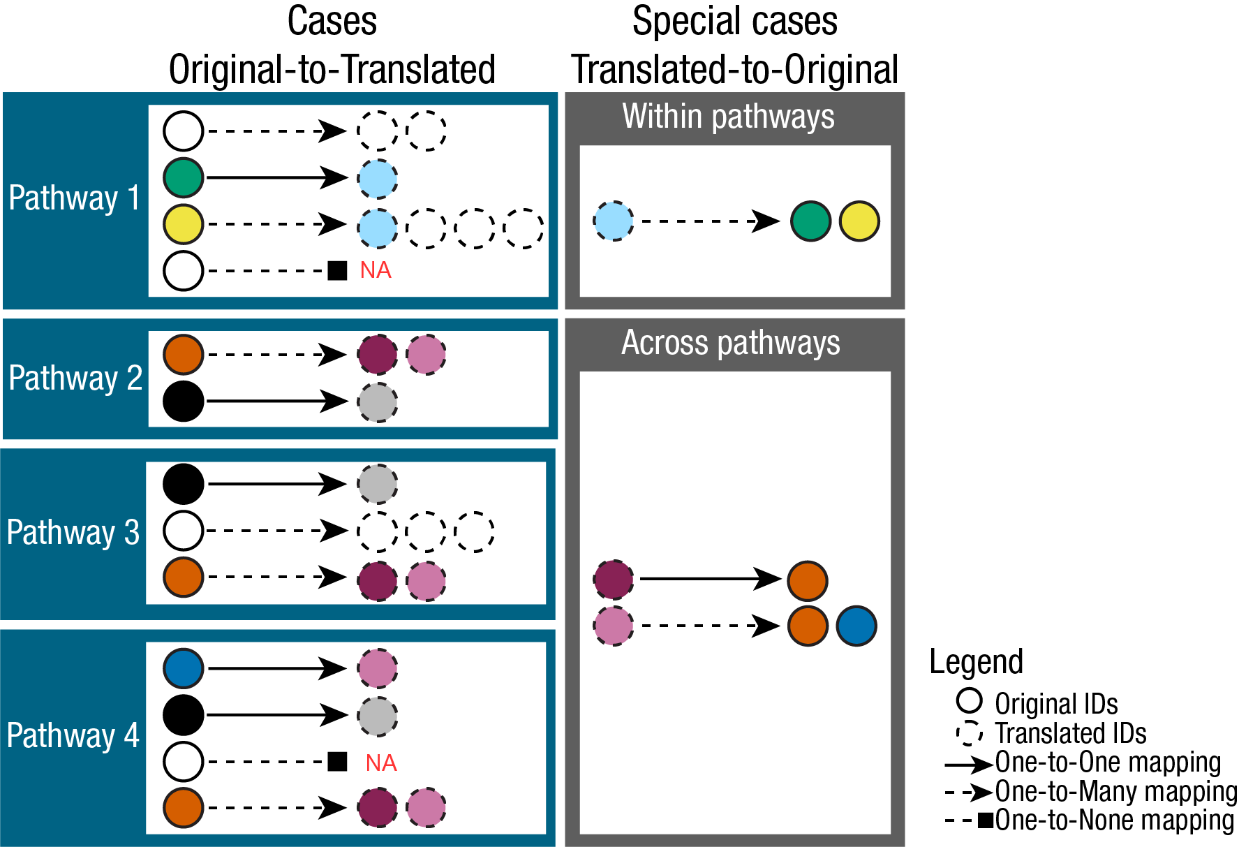
Fig. 2: Mapping problems in prior knowledge metabolite-sets when translating metabolite IDs.

Because of this complexity, the output of translate_id() includes not only the translation table showcased above, but also information about the mapping ambiguity as well as a summary of the relationships between the original and translated IDs.
Indeed, the translation of KEGG to HMDB and PubChem includes multiple data frames, including a summary of the mapping occurrences:

names(KEGG_Pathways_Translated)
#> [1] "TranslatedDF"             "TranslatedDF_MappingInfo"
#> [3] "Mappingsummary_hmdb"      "Mappingsummary_pubchem"

Mappingsummary_hmdb
term	many_to_many	one_to_many	one_to_none	one_to_one	total	to_many	to_none	to_one	to_total	from_many	from_one	from_total	scope
Glycolysis / Gluconeogenesis	12	23	6	13	54	12	6	13	31	6	37	43	group
Citrate cycle (TCA cycle)	0	17	3	9	29	8	3	9	20	0	27	27	group
Pentose phosphate pathway	20	17	10	16	63	11	10	16	37	10	34	44	group
Ascorbate and aldarate metabolism	10	39	26	15	90	16	26	15	57	5	55	60	group
Fatty acid biosynthesis	0	14	46	6	66	6	46	6	58	0	21	21	group
Fatty acid elongation	8	48	11	3	70	25	11	3	39	4	52	56	group

We can also extract a long version of the summary that includes a row for each mapping occurrence, which can be useful for downstream analysis. Yet, this can become very large depending on the amount of many-to-many mappings, hence it is not generated by default. Within translate_id() you can set the parameter summary = TRUE, or, in case you have a data frame that includes both the original and the translated ID, you can use the function mapping_ambiguity() to generate this long summary as well as the mapping summary in general.

# Option 1:
KEGG_Pathways_TranslatedSum <- translate_id(
    data = KEGG_Pathways,
    metadata_info = c(InputID = "MetaboliteID", grouping_variable = "term"),
    from = c("kegg"),
    to = c("hmdb", "pubchem"),
    summary = TRUE
)

# Option 2:
MappingProblems <- mapping_ambiguity(
    data =
        KEGG_Pathways_Translated[["TranslatedDF"]] %>%
        dplyr::rename("KEGG" = "MetaboliteID") %>%
        dplyr::select(Description, KEGG, term, Metabolite, hmdb),
    from = "KEGG",
    to = "hmdb",
    grouping_variable = "term",
    summary = TRUE
)

Long summary of mapping problems taking into account both directions, from-to-to and to-to-from.
KEGG	hmdb	term	KEGG_to_hmdb	Count(KEGG_to_hmdb)	hmdb_to_KEGG	Count(hmdb_to_KEGG)	Mapping
C00002	HMDB0000538	Bacterial secretion system	C00002 –> HMDB0000538, HMDB0257997	2	HMDB0000538 –> C00002	1	one-to-many
C00002	HMDB0000538	Biosynthesis of cofactors	C00002 –> HMDB0000538, HMDB0257997	2	HMDB0000538 –> C00002	1	one-to-many
C00024	HMDB0247926	Ethylbenzene degradation	C00024 –> HMDB0001206, HMDB0247926	2	HMDB0247926 –> C00024	1	one-to-many
C00024	HMDB0247926	Fatty acid degradation	C00024 –> HMDB0001206, HMDB0247926	2	HMDB0247926 –> C00024	1	one-to-many

The table shows that the KEGG ID C00002 maps to 3 different HMDB IDs, and that one of those HMDB IDs, HMDB0000538, maps back to one KEGG ID; hence this mapping is one-to-many. The other two HMDB IDs are also in the table, together with the number of KEGG IDs they map to. Additionally, we have passed grouping_variable = "term" as we have pathways, which means each of those mappings is checked within a pathway and across pathways (e.g. C00002 is shown twice, for two different terms).

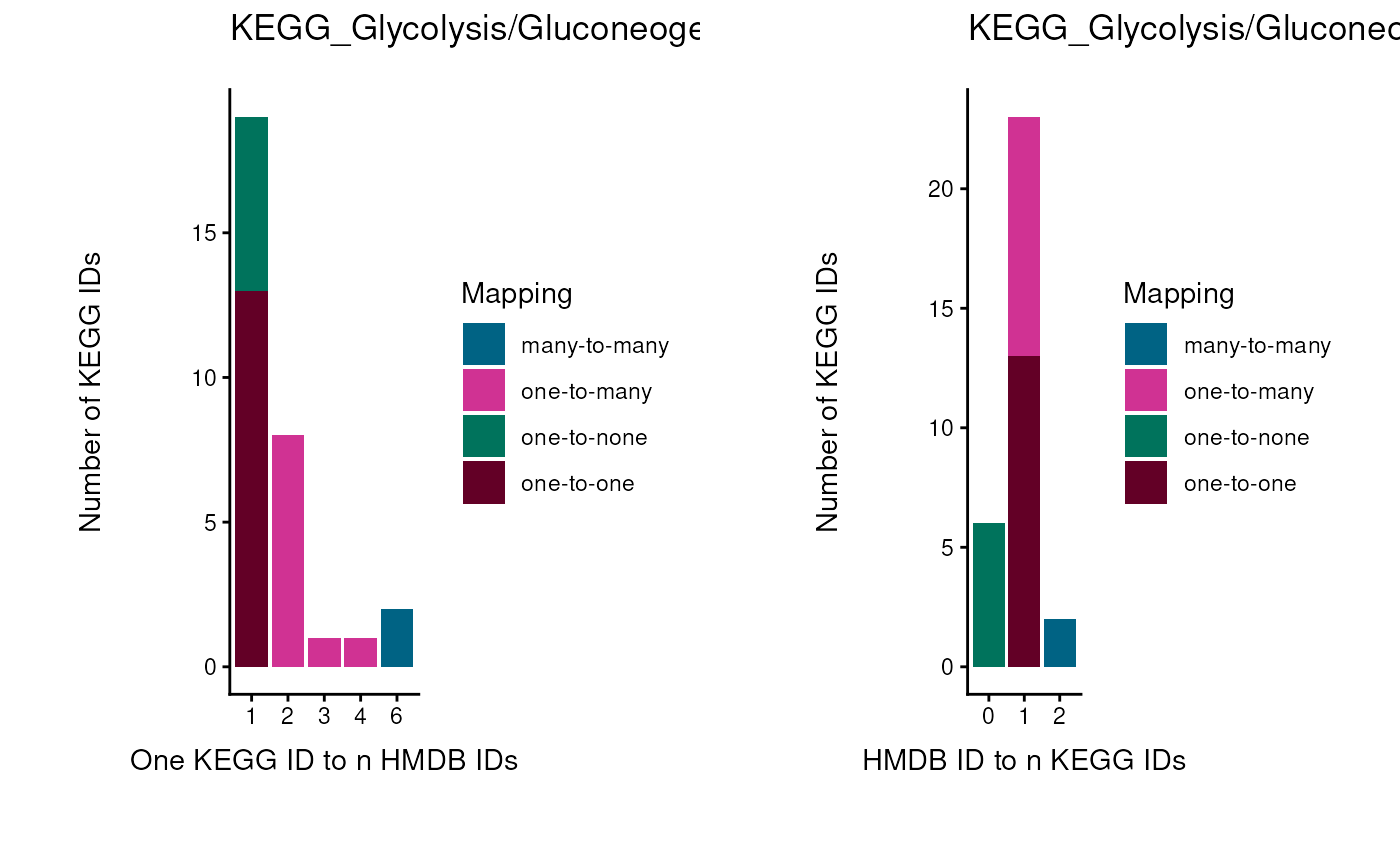
In fact, to perform enrichment analysis we need a column source (e.g. term), and we want to keep the metabolite IDs across pathways consistent, avoid ambiguous mapping (many-to-many mapping) as much as possible, and have this metabolite ID selection guided by the IDs available in our measured input data (Fig. 3). Hence, we can use the measured metabolite IDs to guide the selection of PK IDs. This is crucial to circumvent inflation or deflation of metabolite-sets, which in turn affects the enrichment analysis results.
This is something we are currently working on and hope to provide within the next release, so stay tuned.

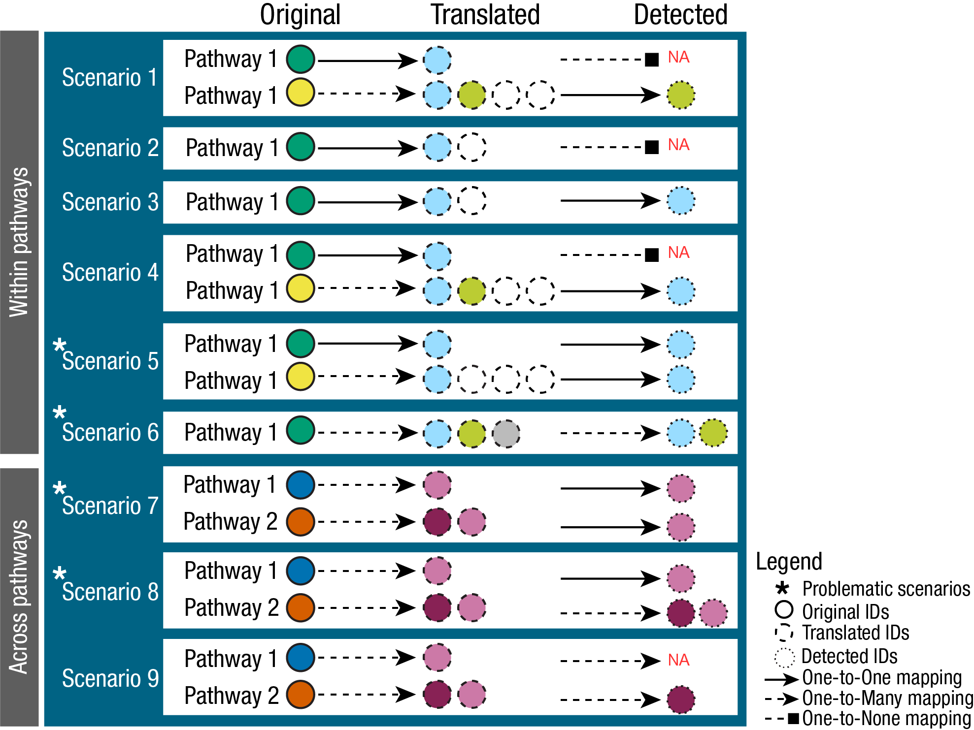
Fig. 3: Mapping problems in prior knowledge metabolite-sets when translating metabolite IDs and the connection to detected (measured input) metabolites.

Pathway coverage of the measured data

Thanks to the translation, the KEGG pathways now carry HMDB IDs, which means we can finally connect them to the Biocrates features. A useful question before any enrichment analysis is: how well does my measured feature space cover each pathway? A pathway of which we measure only a small fraction of metabolites may appear changed because of a single outlier metabolite, whilst a well-covered pathway requires many metabolites to change.

To answer this question in the context of the whole resource, we use cluster_pk(). It computes the similarity between all pairs of pathways based on their shared metabolites, clusters similar pathways, and shows the result as a graph in which each node is a pathway and each edge connects two pathways that share metabolites. Here we only use it as a canvas for our coverage information; the parameters and the interpretation of these graphs for all MetSigDB resources are explained in detail in the MetSigDB vignette.

Compute the pathway coverage

First, we count the metabolites per pathway and determine for each KEGG metabolite whether at least one of its translated HMDB IDs is measured on the Biocrates kit. In line with section 3.4, we use all HMDB IDs of the Biocrates features, not only the first one.

kegg_translated <- KEGG_Pathways_Translated[["TranslatedDF"]] %>%
    group_by(term) %>%
    mutate(n_metabolites_in_pathway = n()) %>% # number of metabolites per pathway term
    ungroup()

# All HMDB IDs measured on the Biocrates kit (multiple IDs per feature are split):
biocrates_hmdb <- FeatureMetadata_Biocrates %>%
    dplyr::filter(!is.na(HMDB), HMDB != "") %>%
    tidyr::separate_rows(HMDB, sep = ",") %>%
    dplyr::mutate(HMDB = stringr::str_trim(HMDB)) %>%
    dplyr::pull(HMDB) %>%
    unique()

# Is each KEGG metabolite detected via any of its translated HMDB IDs?
kegg_metabolite_matches <- kegg_translated %>%
    dplyr::mutate(kegg_row_id = dplyr::row_number()) %>%
    dplyr::select(kegg_row_id, term, n_metabolites_in_pathway, hmdb) %>%
    tidyr::separate_rows(hmdb, sep = ",") %>%
    dplyr::mutate(hmdb = stringr::str_trim(hmdb)) %>%
    dplyr::group_by(kegg_row_id, term, n_metabolites_in_pathway) %>%
    dplyr::summarise(detected_in_biocrates = any(hmdb %in% biocrates_hmdb), .groups = "drop")

# Pathway coverage: what percentage of the metabolites of each KEGG pathway is measured?
pathway_coverage <- kegg_metabolite_matches %>%
    dplyr::group_by(term) %>%
    dplyr::summarise(
        pct_metabolites_detected = 100 * sum(detected_in_biocrates) / dplyr::first(n_metabolites_in_pathway),
        .groups = "drop"
    )

KEGG pathways with the highest coverage by the Biocrates kit.
term	pct_metabolites_detected
Non-alcoholic fatty liver disease	100.0
Serotonin receptor agonists/antagonists	100.0
Leishmaniasis	75.0
Mineral absorption	70.0
Amphetamine addiction	66.7
Cholesterol metabolism	66.7
Cocaine addiction	66.7
GABAergic synapse	66.7
Protein digestion and absorption	62.5
Glutamatergic synapse	60.0

Visualise the coverage in the pathway graph

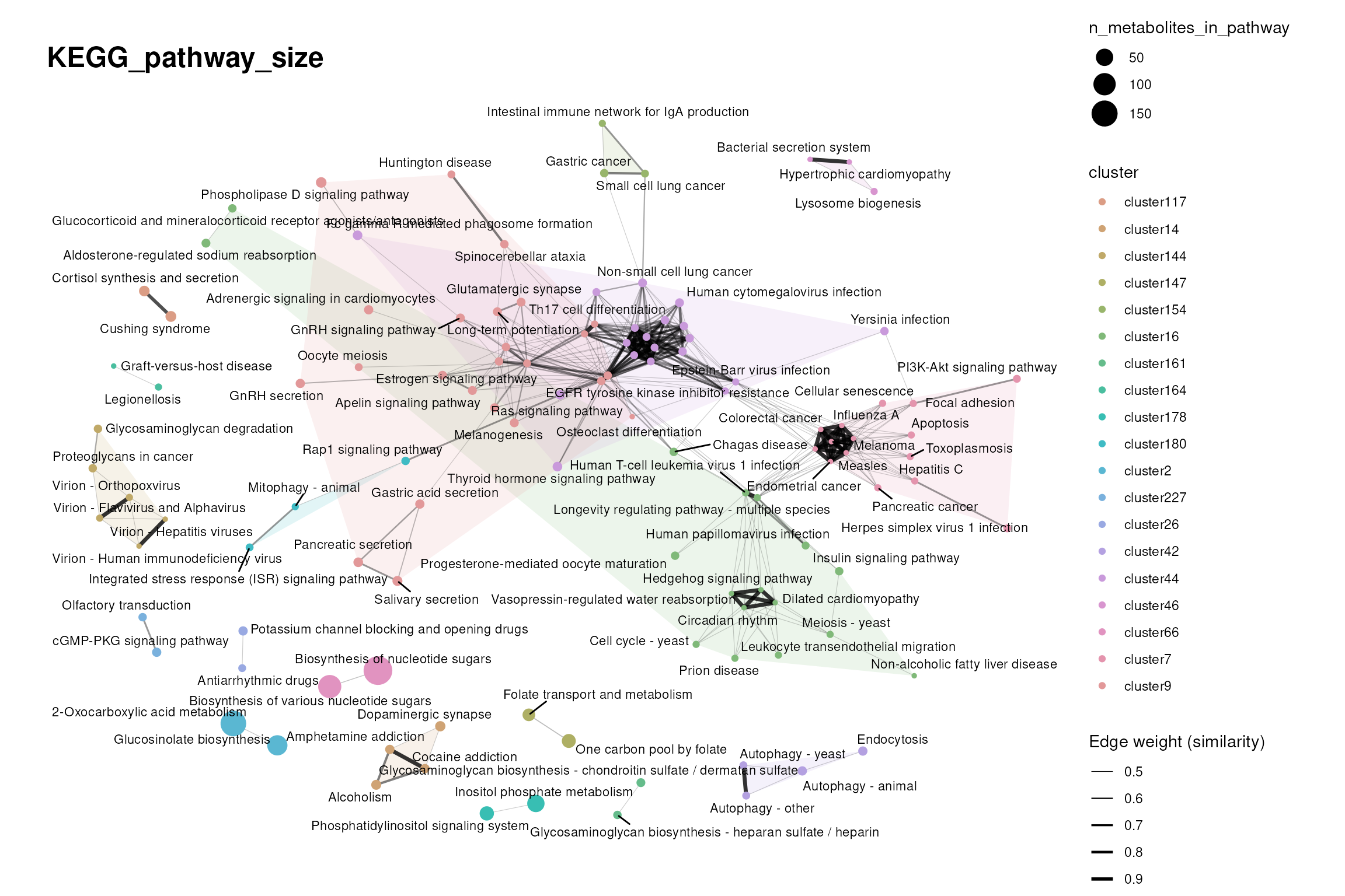
Next, we cluster the KEGG pathways once with cluster_pk(). We then draw the same graph twice with viz_graph(): first with node sizes representing the pathway size (number of metabolites), then with node sizes representing the coverage by the Biocrates kit. As the clustering is identical, only the node sizes differ between the two plots.

set.seed(123)
kegg_clustering <- cluster_pk(
    kegg_translated,
    metadata_info = c(metabolite_column = "MetaboliteID", pathway_column = "term"),
    similarity = "jaccard",
    input_format = "long",
    threshold = 0.4, # only pathways with a similarity above 0.4 are considered for clustering
    clust = "community", # Louvain community detection determines which pathways form a cluster
    save_plot = NULL,
    print_plot = FALSE
)

# Node sizes: pathway size
pathway_size <- kegg_translated %>% dplyr::distinct(term, n_metabolites_in_pathway)
pathway_size <- setNames(pathway_size$n_metabolites_in_pathway, pathway_size$term)
attr(pathway_size, "label") <- "n_metabolites_in_pathway"

# Node sizes: coverage by the Biocrates kit
pathway_coverage_size <- setNames(pathway_coverage$pct_metabolites_detected, pathway_coverage$term)
attr(pathway_coverage_size, "label") <- "pct_metabolites_detected"

set.seed(123)
kegg_graph_size <- viz_graph(
    similarity_matrix = kegg_clustering$similarity_matrix,
    clusters = kegg_clustering$clusters,
    plot_threshold = 0.5, # only pathway-pathway edges with at least 0.5 similarity are plotted
    min_degree = 1,
    node_sizes = pathway_size,
    show_density = TRUE, # coloured background behind clusters
    save_plot = NULL,
    print_plot = TRUE,
    plot_name = "KEGG_pathway_size"
)

set.seed(123)
kegg_graph_coverage <- viz_graph(
    similarity_matrix = kegg_clustering$similarity_matrix,
    clusters = kegg_clustering$clusters,
    plot_threshold = 0.5,
    min_degree = 1,
    node_sizes = pathway_coverage_size,
    show_density = TRUE,
    save_plot = NULL,
    print_plot = TRUE,
    plot_name = "KEGG_pathway_coverage_biocrates"
)

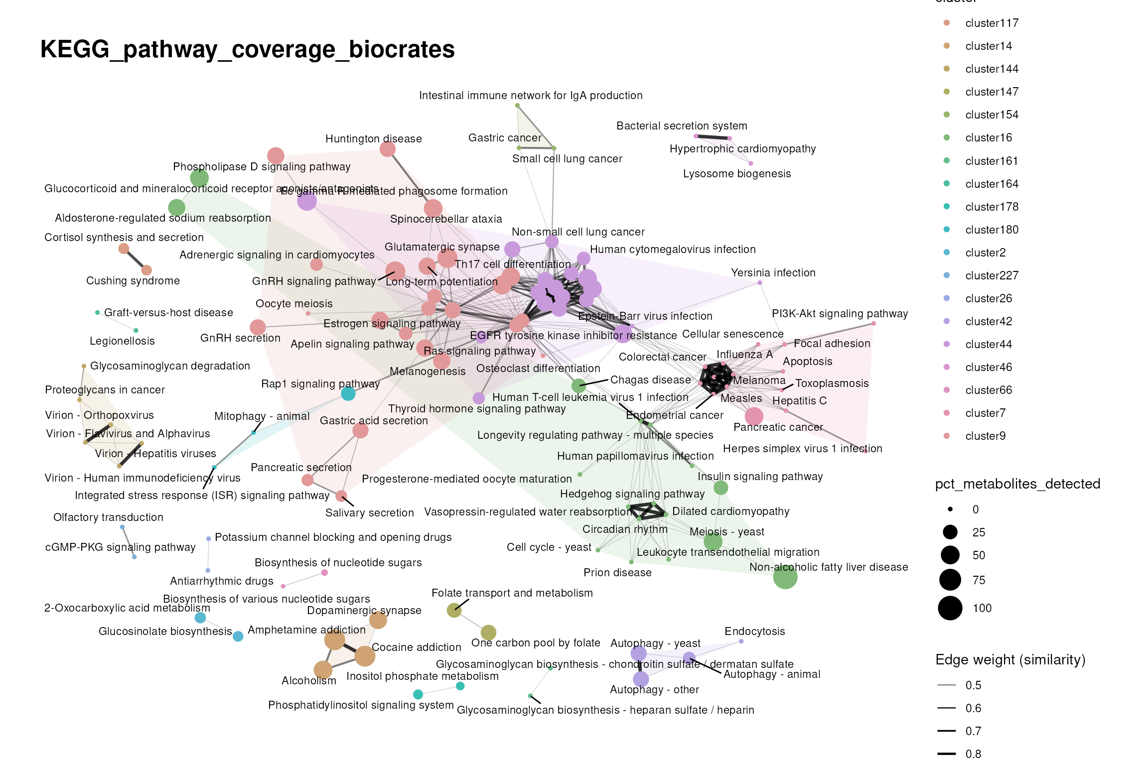
While the clustering stayed the same, the node sizes change, sometimes drastically. Large nodes in the second plot are pathways that are well covered by the Biocrates features. Changes in such well-represented pathways in downstream analyses are more reliable, because a larger number of metabolites must be changed, whilst small nodes (pathways poorly represented by the measured features) may appear changed due to a few outlier metabolites. Comparing both plots also shows that large pathways are not necessarily well covered: the coverage depends on which metabolite classes the measurement platform targets.
Keep in mind that the node size actively changes how we read the graph, so always state what the node size represents when you show such a plot.

Next steps

Now that the measured data is linked to prior knowledge, there are two options to run enrichment analysis:
1. Over Representation Analysis (ORA) that determines if a set of features (e.g. metabolic pathways) is over-represented in a selection of features (e.g. metabolites) from the data in comparison to all measured features, using Fisher’s exact test: cluster_ora(). This can be applied to clusters of metabolites, for example the results of the mca_2cond() or core() functions. If you want more details on these clustering methods, please visit the vignettes Standard Metabolomics or CoRe Metabolomics.

2. Enrichment analysis on standard differential analysis results. We offer ORA with standard_ora(), but there are many other statistical tests that can be used for enrichment analysis. The full scope of different methods is beyond the scope of MetaProViz, but they are available in the decoupleR (Badia-I-Mompel et al. 2022) package from our group.

Before choosing a resource for enrichment analysis, it is worth understanding how the resources differ in size, specificity and redundancy, since this shapes the enrichment results. This is the topic of the follow-up vignette MetSigDB.

Session information

#> R version 4.6.1 (2026-06-24)
#> Platform: x86_64-pc-linux-gnu
#> Running under: Ubuntu 24.04.4 LTS
#> 
#> Matrix products: default
#> BLAS:   /usr/lib/x86_64-linux-gnu/openblas-pthread/libblas.so.3 
#> LAPACK: /usr/lib/x86_64-linux-gnu/openblas-pthread/libopenblasp-r0.3.26.so;  LAPACK version 3.12.0
#> 
#> locale:
#>  [1] LC_CTYPE=en_US.UTF-8       LC_NUMERIC=C               LC_TIME=en_US.UTF-8        LC_COLLATE=en_US.UTF-8    
#>  [5] LC_MONETARY=en_US.UTF-8    LC_MESSAGES=en_US.UTF-8    LC_PAPER=en_US.UTF-8       LC_NAME=C                 
#>  [9] LC_ADDRESS=C               LC_TELEPHONE=C             LC_MEASUREMENT=en_US.UTF-8 LC_IDENTIFICATION=C       
#> 
#> time zone: Etc/UTC
#> tzcode source: system (glibc)
#> 
#> attached base packages:
#> [1] stats     graphics  grDevices utils     datasets  methods   base     
#> 
#> other attached packages:
#> [1] tibble_3.3.1      stringr_1.6.0     dplyr_1.2.1       purrr_1.2.2       rlang_1.3.0       magrittr_2.0.5   
#> [7] MetaProViz_4.99.0 BiocStyle_2.40.0 
#> 
#> loaded via a namespace (and not attached):
#>   [1] splines_4.6.1               later_1.4.8                 R.oo_1.27.1                 cellranger_1.1.0           
#>   [5] polyclip_1.10-7             XML_3.99-0.25               factoextra_2.2.0            lifecycle_1.0.5            
#>   [9] httr2_1.3.0                 tcltk_4.6.1                 rstatix_1.1.0               lattice_0.22-9             
#>  [13] vroom_1.7.1                 MASS_7.3-66                 backports_1.5.1             limma_3.68.5               
#>  [17] sass_0.4.10                 rmarkdown_2.32              jquerylib_0.1.4             yaml_2.3.12                
#>  [21] otel_0.2.0                  zip_3.0.2                   sessioninfo_1.2.4           EnhancedVolcano_1.31.0     
#>  [25] DBI_1.3.0                   RColorBrewer_1.1-3          lubridate_1.9.5             abind_1.4-8                
#>  [29] rvest_1.0.5                 GenomicRanges_1.64.0        R.utils_2.13.0              ggraph_2.2.2               
#>  [33] BiocGenerics_0.58.1         hash_2.2.6.4                tweenr_2.0.3                rappdirs_0.3.4             
#>  [37] IRanges_2.46.0              S4Vectors_0.50.3            ggrepel_0.9.8               pheatmap_1.0.13            
#>  [41] parallelly_1.48.0           pkgdown_2.2.1               svglite_2.2.2               codetools_0.2-20           
#>  [45] DelayedArray_0.38.2         xml2_1.6.0                  ggforce_0.5.0               tidyselect_1.2.1           
#>  [49] farver_2.1.2                viridis_0.6.5               ComplexUpset_1.3.3          matrixStats_1.5.0          
#>  [53] stats4_4.6.1                Seqinfo_1.2.0               jsonlite_2.0.0              tidygraph_1.3.1            
#>  [57] Formula_1.2-6               systemfonts_1.3.2           tools_4.6.1                 progress_1.2.3             
#>  [61] ragg_1.5.2                  Rcpp_1.1.2                  glue_1.8.1                  gridExtra_2.3.1            
#>  [65] SparseArray_1.12.3          xfun_0.61                   decoupleR_2.17.0            qvalue_2.44.0              
#>  [69] MatrixGenerics_1.24.0       ggfortify_0.4.24            withr_3.0.3                 BiocManager_1.30.27        
#>  [73] fastmap_1.2.0               digest_0.6.39               timechange_0.4.0            R6_2.6.1                   
#>  [77] textshaping_1.0.5           colorspace_2.1-3            lpSolve_5.6.23              gtools_3.9.5               
#>  [81] RSQLite_3.53.3              R.methodsS3_1.8.2           tidyr_1.3.2                 generics_0.1.4             
#>  [85] prettyunits_1.2.0           graphlayouts_1.2.5          httr_1.4.9                  htmlwidgets_1.6.4          
#>  [89] S4Arrays_1.12.1             scatterplot3d_0.3-45        inflection_1.3.7            pkgconfig_2.0.3            
#>  [93] gtable_0.3.6                blob_1.3.0                  S7_0.2.2                    XVector_0.52.0             
#>  [97] OmnipathR_4.1.0             htmltools_0.5.9             carData_3.0-6               bookdown_0.48              
#> [101] scales_1.4.0                kableExtra_1.4.1            Biobase_2.72.0              knitr_1.52                 
#> [105] rstudioapi_0.19.0           tzdb_0.5.0                  reshape2_1.4.5              rjson_0.2.23               
#> [109] checkmate_2.3.4             curl_8.0.0                  cachem_1.1.0                Polychrome_1.6.2           
#> [113] parallel_4.6.1              vipor_0.4.7                 cosmosR_1.20.0              desc_1.4.3                 
#> [117] pillar_1.11.1               grid_4.6.1                  logger_0.4.3                vctrs_0.7.3                
#> [121] ggpubr_1.0.0                car_3.1-5                   beeswarm_0.4.0              evaluate_1.0.5             
#> [125] readr_2.2.0                 cli_3.6.6                   compiler_4.6.1              crayon_1.5.3               
#> [129] ggsignif_0.6.4              labeling_0.4.3              plyr_1.8.9                  fs_2.1.0                   
#> [133] ggbeeswarm_0.7.3            writexl_2.0.1               stringi_1.8.9               viridisLite_0.4.3          
#> [137] BiocParallel_1.46.0         Matrix_1.7-6                hms_1.1.4                   patchwork_1.3.2            
#> [141] bit64_4.8.6                 ggplot2_4.0.3               statmod_1.5.2               SummarizedExperiment_1.42.0
#> [145] CARNIVAL_2.22.0             igraph_2.3.4                broom_1.0.13                memoise_2.0.1              
#> [149] bslib_0.12.0                bit_4.6.0                   readxl_1.5.0.1

Bibliography

Badia-I-Mompel, Pau, Jesús Vélez Santiago, Jana Braunger, et al. 2022. “decoupleR: Ensemble of Computational Methods to Infer Biological Activities from Omics Data.” Bioinformatics Advances 2 (1): vbac016. https://doi.org/10.1093/bioadv/vbac016.

Braisted, John, Andrew Patt, Cole Tindall, et al. 2023. “RaMP-DB 2.0: A Renovated Knowledgebase for Deriving Biological and Chemical Insight from Metabolites, Proteins, and Genes.” Bioinformatics, no. 1 (January). https://doi.org/10.1093/bioinformatics/btac726.

Castanza, Anthony Scott, Jill Marie Recla, David Eby, Helga Thorvaldsdottir, Carol J. Bult, and Jill P Mesirov. 2022. “The Molecular Signatures Database Revisited: Extending Support for Mouse Data.” BioRxiv, ahead of print, October. https://doi.org/10.1101/2022.10.24.513539.

Dugourd, Aurelien, Christoph Kuppe, Marco Sciacovelli, et al. 2021. “Causal Integration of Multi-Omics Data with Prior Knowledge to Generate Mechanistic Hypotheses.” Molecular Systems Biology, no. 1 (January): e9730. https://doi.org/10.15252/msb.20209730.

Farr, Elias, Daniel Dimitrov, Christina Schmidt, et al. 2024. “MetalinksDB: A Flexible and Contextualizable Resource of Metabolite-Protein Interactions.” Briefings in Bioinformatics, no. 4 (May). https://doi.org/10.1093/bib/bbae347.

Gaude, Edoardo, and Christian Frezza. 2016. “Tissue-Specific and Convergent Metabolic Transformation of Cancer Correlates with Metastatic Potential and Patient Survival.” Nature Communications 7 (October): 13041. https://doi.org/10.1038/ncomms13041.

Jaccard, Paul. 1901. Étude Comparative de La Distribution Florale Dans Une Portion Des Alpes Et Du Jura. https://doi.org/10.5169/SEALS-266450.

Kanehisa, M, and S Goto. 2000. “KEGG: Kyoto Encyclopedia of Genes and Genomes.” Nucleic Acids Research 28 (1): 27–30. https://doi.org/10.1093/nar/28.1.27.

Liberzon, Arthur, Chet Birger, Helga Thorvaldsdóttir, Mahmoud Ghandi, Jill P Mesirov, and Pablo Tamayo. 2015. “The Molecular Signatures Database (MSigDB) Hallmark Gene Set Collection.” Cell Systems 1 (6): 417–25. https://doi.org/10.1016/j.cels.2015.12.004.

Sciacovelli, Marco, Aurelien Dugourd, Lorea Valcarcel Jimenez, et al. 2022. “Dynamic Partitioning of Branched-Chain Amino Acids-Derived Nitrogen Supports Renal Cancer Progression.” Nature Communications 13 (1): 7830. https://doi.org/10.1038/s41467-022-35036-4.

Prior Knowledge - Access & Integration

Christina Schmidt

Jannik Franken

Macabe Daley